Introduction to the course. We went through the syllabus. Everyone introduced themselves, said a few interesting things, and filled out the first-day questionnaire. Near the end of class, we discussed the following question: Is it possible to cover an 8 × 8 chessboard with dominoes, if the two corner squares are missing?
Handouts: Syllabus (PDF, TeX); first-day questionnaire (PDF, TeX).
Read for next class: Thinking Mathematically, through page 10.
Do for next class: Find my office; try “Paper Strip” (Thinking Mathematically, page 4).
We discussed “Paper Strip” and several different ways the problem might be approached. We reviewed the chessboard/domino problem and used the idea of coloring to answer the following question: If a mouse is in the upper left corner square of a 4 × 3 grid, and moves around by choosing a neighboring square at random, what is the probability that the mouse will be in the lower right corner square after 20 moves?
Homework: Assignment 1 (PDF, TeX), due Wednesday, January 20.
Read for next class: Thinking Mathematically, through page 25.
Do for next class: Try to extend “Palindromes” (Thinking Mathematically, page 5) in an interesting way.
We began by discussing some extensions to “Palindromes” that students investigated. Several people noticed that, apparently, every palindrome with an even number of digits is divisible by 11. Why is this? Another conjecture was that multiplying a four-digit palindrome by 11 produces another palindrome, except when the middle digits are 9’s; and dividing a four-digit palindrome by 11 produces another palindrome, except when the middle digits are 1’s or 0’s. Is this true? If so, why?
For the next several classes we are going to be talking about shapes and
geometry. We started this topic with an introduction to
polyominoes. The first question we
investigated was whether we can use “bent” trominoes
( )
to tile an 8 × 8 checkerboard with one square missing. We
saw a very clever argument that showed it is always possible, no matter
which square is removed; the argument first showed it was possible to tile
a 2 × 2 checkerboard with one missing square, and then a
4 × 4 checkerboard with one missing square (by dividing it
into four 2 × 2 checkerboards), in order to prove the claim
for the 8 × 8 checkerboard.
)
to tile an 8 × 8 checkerboard with one square missing. We
saw a very clever argument that showed it is always possible, no matter
which square is removed; the argument first showed it was possible to tile
a 2 × 2 checkerboard with one missing square, and then a
4 × 4 checkerboard with one missing square (by dividing it
into four 2 × 2 checkerboards), in order to prove the claim
for the 8 × 8 checkerboard.
We then made a list of all the free pentominoes (there are 12 of them) and looked at the difference between fixed polyominoes, one-sided polyominoes, and free polyominoes. There are many questions on the polyominoes handout given in class; we will look at some of these on Wednesday.
Handout: Polyominoes worksheet, graph paper.
Read for next class: Problem Solving Through Recreational Mathematics, introduction to Chapter 8 (page 273), sample problems (pages 274–275), and the section about polyominoes and Soma (pages 281–285).
Do for next class: The first homework is due on Wednesday, January 20 (which is our next class—we do not meet on Monday). Also, try two or three of the questions from the polyominoes handout. There are many questions for you to try; find a couple that seem interesting to you. Bring graph paper and your polyomino cutouts to class on Wednesday, because we will continue to play with polyominoes.
Martin Luther King, Jr. Day; no class today.
Today we talked about polyominoes. One observation that had been made over the weekend was that the number of ways to tile a 2 × n checkerboard with dominoes follows the pattern of the Fibonacci numbers, and we saw why this was the case.
We then worked in groups, investigating various questions about polyominoes. We found that there were 35 free hexominoes (and listed them all). One group examined the perimeters of polyominoes, and found that the perimeter of a polyomino is always even. Another group played the two-player pentomino game described in the handout, and tried to find a good strategy. A third group discovered that some of the hexominoes can be built from two trominoes, and some can be built from three dominoes; some can be built in both ways, but some can be built in neither of these ways. One group explored the question of which polyominoes can be used to tile the plane. Near the end of class a couple of people considered extending the idea of polyominoes to three dimensions by building shapes out of cubes.
A friend sent me a link to a page that has a really cool “Tetris Tiler,” which attempts to use free tetrominoes to tile a checkerboard with some missing squares. The program is smart enough to try the difficult areas on the board first; this is why the first few pieces are sometimes placed in very different locations. Try playing around with this a bit—it’s pretty interesting.
Read for next class: Thinking Mathematically, pages 26–38.
Class was canceled today due to an unconfirmed security and safety threat to Wean Hall. We will meet again on Monday, January 25.
Today we talked about working systematically. As an example I described the method I used to list the 35 free hexominoes. We also discussed the very useful technique called backtracking, using the eight queens puzzle as an example.
Homework: Assignment 2 (PDF, TeX), due Monday, February 1.
Handout: Working systematically.
Read for next class: Working systematically handout; Thinking Mathematically, pages 38–48.
Do for next class: Try solving the eight queens problem or tackling one of the applications of backtracking described in the handout. Take a look at the “Tetris Tiler” or the maze generator, both of which use backtracking techniques to solve puzzles.
We talked about symmetry and tilings today. (A handout about these topics will be posted eventually.) We began by identifying four types of symmetry: reflection symmetry, rotation symmetry, translation symmetry, and glide symmetry. Only reflection and rotation symmetry apply to finite shapes; translation and glide symmetry require infinite shapes (such as a tiling of the plane). Reflection symmetry implies one or more lines of symmetry, while rotation symmetry implies a point of symmetry and a (smallest) angle of rotation. Shapes can be classified according to their symmetry; to do so (for finite shapes, like polygons), you need to count the number of lines of (reflection) symmetry, if any, and determine the (smallest) angle of rotation symmetry, if any.
We began our discussion of tilings, also called tessellations, with some geometric definitions: polygon, regular polygon, convex polygon, vertex, and interior and exterior angles. We derived some formulas for the measure of interior and exterior angles of regular polygons. We then saw how any triangle, any parallelogram, and in fact any quadrilateral can tile the plane. Finally we introduced some classifications for infinite tilings of the plane: edge-to-edge tilings, uniform tilings, regular tilings, and semiregular tilings.
We will continue talking about tilings on Friday, including some methods of modifying a fundamental tiling to form a more interesting and artistic tiling. At this point you should be able to work on every problem from Homework 2 except Problem 5. Also on Friday we will review a bit of algebra and discuss Chapter 3 from Problem Solving Through Recreational Mathematics.
Handout: Solutions to Homework 1 (PDF, TeX; MetaPost drawings: cube, star, tepee, tetrahedron).
Read for next class: Chapter 3 of Problem Solving Through Recreational Mathematics, pages 70–84.
Today we finished talking about tilings. We reviewed the concepts that were introduced on Wednesday. We saw why there are only three regular tilings, and we drew an example of a semiregular tiling. In the last part of the class, we looked at how a basic tiling can be modified to form a tiling that uses more complicated shapes. (This is the idea behind Question 5 of Homework 2.)
We didn’t get to algebra today; we’ll talk about that on Monday, when we’ll talk about Chapter 3 from Problem Solving Through Recreational Mathematics.
I will write a handout about symmetry and tilings this weekend. When I get it done, I will post a link to it on the course home page. I will also hand out paper copies on Monday. Since I feel I owe you something in writing about symmetry and tilings before the homework is due, we decided to push back the due date for Homework 2 to Wednesday, February 3.
Read for next class: Chapter 3 of Problem Solving Through Recreational Mathematics, pages 70–84.
Do for next class: Problems 3.3 and 3.9 from Chapter 3 of Problem Solving Through Recreational Mathematics, page 70–85.
The first thing I did today was to give a handout about symmetry and tilings to complement the things we talked about in class last Wednesday and Friday. If anything in the handout seems unclear, incomplete, or confusing, please let me know and I will be happy to answer your questions.
The reading for today was Chapter 3 from Problem Solving Through Recreational Mathematics, which is titled “From Words to Equations: Algebraic Recreations.” We discussed problems 3.3 and 3.9. I briefly showed how to draw a regular hexagon with a ruler and compass (here’s a YouTube video that explains it too); an equilateral triangle can be drawn in a similar way.
We talked about the use of algebraic variables to represent unknown quantities and the importance and significance of a unique solution to an algebraic problem (and the possible existence of extraneous solutions). We considered the meaning of the equals sign (it means “equals” or “is”, not “therefore” or anything else). We examined some common algebraic mistakes (resist the temptation of the freshman’s dream—don’t forget to FOIL when multiplying polynomials; remember to flip the sign of an inequality if you multiply or divide by a negative number). We reviewed methods for solving quadratic equations (using the quadratic formula) and systems of equations (by substitution or elimination), with a side note about the story of Évariste Galois. We also noted the important fact that you can’t average averages and explored the idea of dimensional consistency.
Handout: Symmetry and tilings.
Read for next class: Chapter 3 of Problem Solving Through Recreational Mathematics, pages 70–84 (if you haven’t already).
Do for next class: Homework 2.
Today we did some more algebra puzzles; see the handout (PDF). At the end of class we talked about a method to find a formula for a sequence of numbers: Take the differences between successive numbers in the sequence, then the differences between the differences, and so on, until a row of constant differences is reached (if this happens at all). The number of times you have to take differences is the likely degree of the formula for the numbers. For example, if constant differences appear on the first row, the formula is likely to be a linear function; if they appear on the second row, it is likely to be a quadratic function; and so on. Then you can use the general form of a function of that degree (for example, the general form of a quadratic function is y = ax2 + bx + c) and plug in several values of x and y from the given sequence to form a system of equations, which you can then solve for the unknown coefficients (a, b, c, etc.).
Handout: Algebra puzzles (PDF, TeX).
Read for next class: The first part of Chapter 4 in Problem Solving Through Recreational Mathematics, pages 100–108.
Do for next class: Problem Solving Through Recreational Mathematics, problem π (that is, problem 3.14). Note the H and A symbols next to the problem number; these indicate, respectively, that a hint and an answer can be found in the back sections of the book. For a challenge, try problem 3.19.
We reviewed the method presented on Wednesday for finding a formula for a sequence of numbers, and we went through a solution of problem 3.14 from Problem Solving Through Recreational Mathematics. We then started Chapter 4, about number theory. Today we talked briefly about Diophantine equations, which are equations that require the solutions to be integers. For example, an equation in which x represents the number of marbles in a bag is probably a Diophantine equation, because it doesn’t make sense to have a fractional number of marbles.
We also talked a bit about Fermat’s Last Theorem, a very famous problem in number theory that remained unsolved for over 350 years until Andrew Wiles finally completed the proof in the 1990s. Fermat’s Last Theorem states that the Diophantine equation an + bn = cn has no positive integer solutions if n ≥ 3. Of course, if n = 2 this equation becomes a2 + b2 = c2, which is the equation found in the Pythagorean theorem. There are many positive integer solutions to this equation, called Pythagorean triples; one example is a = 3, b = 4, c = 5. Extending a Pythagorean triple into three dimensions gives an Euler brick, a rectangular brick with integer side lengths and integer face diagonals. One open question is whether there is any Euler brick that also has an integer body diagonal (the line from one corner of the brick through the center to the opposite corner). Such an object is called a perfect cuboid; no one has ever discovered such a thing, but no one knows any reason it shouldn’t exist.
We will continue our discussion of Chapter 4 on Monday, talking about divisibility and prime numbers.
Challenge questions: PDF, TeX.
Homework: Assignment 3 (PDF, TeX; MetaPost drawings: one point, two points, three points, four points, five points), due Friday, February 12.
Read for next class: The first part of Chapter 4 in Problem Solving Through Recreational Mathematics, pages 100–108.
Do for next class: Problem Solving Through Recreational Mathematics, problem 3.5.
All classes were canceled today due to the recent heavy snowfall. We will meet again on Wednesday, February 10.
Classes were canceled again today since many city streets are still in poor condition. We will meet again on Friday, February 12.
Amazingly we had class today. The due date for Homework 3 has been pushed back to next Wednesday, February 17. Here are a few hints for problem 7 on the homework: The handout given today might be helpful; when n = 10, there are 256 regions (you can use this to check your formula); be sure to draw your points so that no three chords intersect in a single point.
We spent the first part of class discussing problem 3.5 from Problem Solving Through Recreational Mathematics. There is a very short and efficient solution presented in the back of the book; I presented my own solution, which was more circuitous but produced the same answer. We then spent a bit of time talking about finding a formula for a sequence of numbers, which was presented last Wednesday and Friday. We also explored the connections between this method of guessing a formula and the concept of mathematical proof: usually answers to problems begin as conjectures (guesses) before they are proven and become theorems. We will see more of this idea throughout the rest of the course.
Next we returned to the topic of number theory that we began last Friday. We discussed the definition of divisibility (see Definition 4.2 on page 104 of the textbook) and investigated a few examples. We concluded by mentioning some divisibility rules, which can be used to quickly test for divisibility by certain small integers. Finally, I handed out early course feedback forms to gather comments about how the course is going so far.
Handout: Finding a formula for a sequence of numbers, early course feedback form.
Read for next class: Handout from today, and the next part of Chapter 4 in Problem Solving Through Recreational Mathematics, pages 108–119.
Do for next class: Problem Solving Through Recreational Mathematics, problems 4.5 and 4.11.
Today we discussed divisibility (in particular, Theorem 4.1 from Problem Solving Through Recreational Mathematics) and prime numbers (the definition and Theorem 4.2). We then used the sieve of Eratosthenes (pages 107–108) to find the prime numbers less than 32.
On Wednesday we will talk some more about prime numbers, including a beautiful proof that there are infinitely many of them.
Handout: List of potential topics, so that you can get an overall idea of where this class might be headed.
Read for next class: Problem Solving Through Recreational Mathematics, pages 108–119.
Do for next class: Problem Solving Through Recreational Mathematics, problems 4.5 and 4.11.
We began class today by seeing solutions to problems 4.5 and 4.11 from Problem Solving Through Recreational Mathematics. We then went through Euclid’s proof that there are infinitely many prime numbers, which is a classic example of a proof by contradiction, in which a theorem is proved to be true by showing that a logical contradiction would result if it were false. (This proof is given on pages 106 and 107 of Problem Solving Through Recreational Mathematics.)
We briefly discussed the complementary ideas of least common multiple (lcm) and greatest common divisor (gcd). The least common multiple of two positive integers is the smallest number that is a multiple of both of them. For example, the least common multiple of 10 and 12, written lcm(10, 12), is 60: first, 60 is a multiple of 10 (because 10 × 6 = 60), and also 60 is a multiple of 12 (because 12 × 5 = 60), and it is the smallest number that is a multiple of both of them. The greatest common divisor of two positive integers is the largest number that is a divisor (factor) of both of them. For example, the greatest common divisor of 10 and 12, written gcd(10, 12), is 2: certainly 2 is a divisor of both 10 and 12 (10 = 2 × 5 and 12 = 2 × 6), and no larger number is a divisor of both of them. We observed that the numbers in this example have an interesting property: the product of the two numbers is 10 × 12 = 120, and the product of their lcm and gcd is 60 × 2 = 120. Is this always true? See page 116 of Problem Solving Through Recreational Mathematics for the definition of greatest common divisor (though least common multiple is strangely absent).
I spent a few minutes at the end talking in very broad terms about the applications of prime numbers to modern cryptography, including data security on the Internet. Essentially these cryptographic methods rely on the fact that multiplying numbers is easy, but factoring numbers (the “opposite” of multiplication, in a way) is hard.
Handout: Homework 2 solutions (PDF, source files).
Do for next class: Relax.
I handed out Homework 4 today; it is due next Friday. I considered asking you to do five questions, but I decided to leave it at four. However, I encourage you to try to do at least five of them if you can. Your grade will be based on your best four.
Today we discussed some additional topics in number theory that are not in the textbook. We began by very briefly reviewing the concepts of greatest common divisor and least common multiple introduced on Wednesday. Then we went through an example of the Euclidean algorithm, which is a process to find the greatest common divisor of two numbers. In the course of this we saw how to find remainders with a calculator. We then talked about deficient, abundant, and perfect numbers. Finally we discussed Mersenne numbers and Fermat numbers, the relationships between Mersenne primes and perfect numbers, and some of the open questions that surround these topics.
Homework: Assignment 4 (PDF, TeX; MetaPost drawing: sheep pen), due Friday, February 26.
Handout: Additional topics in number theory.
Read for next class: Problem Solving Through Recreational Mathematics, page 119 through the top of page 125.
I began today by taking care of a few loose ends from last Friday. First I gave a geometric explanation for why the Euclidean algorithm works; the idea is from the worked example in Wikipedia’s article about the Euclidean algorithm. I also briefly mentioned Fermat’s little theorem and its usefulness in identifying numbers as composite; such tests for compositeness are important in modern cryptographic techniques.
Today’s focus was on congruence and modular arithmetic, which are fancy terms for working with remainders. We saw how working with remainders is like working with times on a clock: If it is 10:00 now, in 5 hours it will be 3:00; so in some sense we can say that “10 + 5 = 3.” (This equation is true, as long as we are working with remainders after division by 12.) We reviewed the basic parts of a division problem (dividend, divisor, quotient, and remainder) and the relationships between them; see The Math Page or TutorNext for a refresher. In particular, when the divisor is d, the possible remainders are 0 through d − 1. Theorem 4.7 in Problem Solving Through Recreational Mathematics describes the division process algebraically.
We introduced the notation a ≡ b (mod d), read “a is congruent to b mod d,” which means that a and b have the same remainder when they are divided by d. (The word “mod” is short for the Latin word “modulo,” which is used to indicate the divisor, or “modulus,” with which we are working.) We then saw that, for a fixed value of d, the remainders after division by d repeat in a cycle as we go up the number line. Continuing this cycle, we can meaningfully assign remainders to negative numbers, too; for example, the remainder when −3 is divided by 5 is 2, because −3 = 5(−1) + 2. (Remember that remainders after division by d must be between 0 and d − 1.) Therefore we can classify all the integers into remainder classes, according to the remainder they give when divided by d. For instance, modulo 5 (that is, working with remainders after division by 5), the remainder class 2 consists of all integers that give a remainder of 2 when divided by 5: this remainder class is the set of integers {…, −18, −13, −8, −3, 2, 7, 12, 17, …}.
The main point of modular arithmetic, which is embodied in Theorem 4.8 in Problem Solving Through Recreational Mathematics, is that we can add, subtract, and multiply with remainders (strictly speaking, with remainder classes) as if they were numbers.
On Wednesday we will revisit these ideas and do some more examples to help illustrate what is going on. Congruence and modular arithmetic together form perhaps the most useful concept in number theory, and they have wide applications throughout all of mathematics, so it is very helpful to be comfortable with them.
Read for next class: The rest of Chapter 4 in Problem Solving Through Recreational Mathematics, pages 125–138. (This is optional reading. It discusses a method for solving linear Diophantine equations. I will present a different method based on the Euclidean algorithm on Wednesday or Friday.)
Do for next class: Problem Solving Through Recreational Mathematics, problem 4.21.
At the beginning of class today some people said they would like more time to work on Homework 4, so if you'd like to turn it in on Monday instead of Friday, that's fine.
Today we discussed modular arithmetic again. In modular arithmetic, we are ignoring the actual values of numbers and are only considering the remainder after division by some fixed number (called the modulus). We did some examples of addition and multiplication mod 7, and then tackled the following question: What is the last digit of 176?
Handout: Homework 3 solutions (PDF, source files).
Read for next class: Chapter 3 in Thinking Mathematically, pages 49–62.
Do for next class: “Diagonals of a Rectangle,” on page 166 of Thinking Mathematically.
Today we did a few more examples of modular arithmetic with remainders after division by 4, that is, arithmetic mod 4. We then went through an example of the extended Euclidean algorithm, which can be used to solve linear Diophantine equations in two variables; see the handout for more information. Finally we talked a little bit about Chapter 3 from Thinking Mathematically. Think about the problems in this chapter and the problem called “Diagonals of a Rectangle” on page 166 for class on Monday.
Handout: The extended Euclidean algorithm.
Read for next class: Extended Euclidean algorithm handout; Chapter 3 in Thinking Mathematically, pages 49–62.
Do for next class: “Diagonals of a Rectangle,” on page 166 of Thinking Mathematically.
We spent today working in groups on five problems I presented at the beginning of class. The first four problems were from Thinking Mathematically (“Threaded Pins,” page 52; “Leapfrogs,” page 57; “Cartesian Chase,” page 162; and “Thirty-one,” page 197), while the last was a problem I heard from a friend last year:
You have an n × n chessboard and a marker. You begin by marking an X through some of the squares of the chessboard. Next, you mark an X through all of the squares which share at least two sides with squares already containing an X. You continue marking an X through such squares until there are no more unmarked squares that share at least two sides with marked squares. (Note that adding an X may open the possibility for another X to be added.)
Sometimes when you do this, every square on the board will be marked with an X. Other times, the process will stop with some empty squares left over. In terms of n, what is the minimum number of marked squares you can start with and still end up with every square on the board marked with an X?
See the picture below for the process on a 5 × 5 chessboard with a certain four squares initially marked. In the end, a total of eight squares are marked.
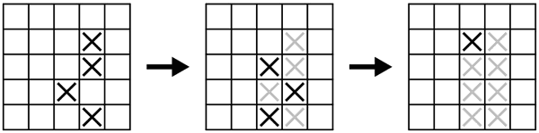
Several people decided that the answer to this puzzle is n. How can it be done with n squares initially marked? Can you find a reason that it cannot be done with fewer than n squares initially marked? (Hint: Perimeter.)
Read for next class: The first part of Chapter 4 in Thinking Mathematically, pages 63–67.
Do for next class: Ponder the problems in the reading.
Today we again worked in small groups on some puzzles. See the handout for the list. (The first five are the same puzzles we thought about on Monday; the other six are new.)
Handout: Spring break puzzles (PDF, TeX; MetaPost drawings: Xs on a chessboard, grid sums).
Read over spring break: The handout from today.
Do over spring break: Figure out some of these puzzles.
Spring break. Have fun on the beach with some spring break puzzles.
We spent today thinking about a problem from Thinking Mathematically, “Nullarbor Plain” on page 183. We weren’t able to solve the problem completely in the time we had, though we were able to establish a few facts and make a couple of conjectures. If you have a chance to think about this problem, see where you can go with it.
Homework 5 was handed out today. Note that the problems are divided into two parts. Part A consists of the problems I thought were more or less straightforward; Part B is the problems that will probably require more creative thinking. At least one of the problems you turn in should be from Part B.
On Wednesday we will start discussing set theory. From there we will explore counting and combinatorics, graph theory, and probability.
Handout: Solutions to Homework 4 (PDF, TeX; MetaPost drawing: sheep pen).
Homework: Assignment 5 (PDF, TeX), due Wednesday, March 24.
Read for next class: Chapter 4 in Thinking Mathematically, pages 67–84.
Do for next class: Think about “Nullarbor Plain” or one of the problems from the reading (“Square Differences” on page 78 or “Fifteen” on page 79).
The project was handed out today. It is due on the last day of class. See the project handout for more details. If you would like to do something other than (or in addition to) the suggestions in the handout, please come talk to me. When you have decided on a project group, please e-mail me to let me know.
We began discussing set theory today. We covered the basic definitions and notation, sets containing other sets, cardinality, and the empty set, and about half of what I want to say about subsets. We’ll continue with sets on Friday.
Handouts: Project (PDF, TeX); how to avoid plagiarism (PDF, TeX); sets.
Read for next class: Handout about sets.
Do for next class: Decide about your project group.
We continued with set theory today, covering subsets, sets of numbers, set-builder notation, unions and intersections, and a bit about Venn diagrams. We will finish discussing set theory on Monday, after which we will begin combinatorics and counting.
Handout: Venn diagrams and questions.
Read for next class: Handout about sets, including the section on Venn diagrams.
Do for next class: Answer the questions at the end of the sets handout.
Today we finished discussing set theory. We covered the various set operations and how they are represented with Venn diagrams. At the end of class I presented the story of Hilbert’s hotel, which demonstrates a very counterintuitive result about infinite sets. We will talk about this a little more on Wednesday and then discuss combinatorics and counting.
Read for next class: Handout about sets, if you haven’t already.
Do for next class: Homework 5.
We talked about counting today. We discussed the addition principle, the principle of inclusion–exclusion, the multiplication principle, and permutations. We also counted the number of ways to choose r elements from a set of size n in two different cases: one in which replacement is allowed and the order of the choices is important, and the other in which replacement is not allowed and the order is important. We will finish talking about counting on Friday.
Read for next class: Counting handout.
Do for next class: Relax.
We finished talking about counting today. We counted the number of ways to choose r elements from a set of size n without replacement, when the order of the choices is not important. We also discussed the pigeonhole principle and the idea of “reading” a mathematical expression as a description of a selection process.
Homework: Assignment 6 (PDF, TeX; MetaPost drawings: streets, chords), due Monday, April 5.
Read for next class: The first part of Appendix C in Problem Solving Through Recreational Mathematics, pages 337–349.
Do for next class: Practice Problem C.K.2(a) in Problem Solving Through Recreational Mathematics, page 349.
Today we did an experiment to test the solution of the Monty Hall problem. Our results were not exactly what is predicted by theory (we won with probability 1/9 when we stayed with our original choice and with probability 3/7 when we switched), but did go to show that it is advantageous to switch. We then discussed a little about the philosophy of probability, contrasting the frequentist interpretation (which envisions probabilities as representing expected results of many repeated trials) with the Bayesian interpretation (which views probabilities as measures of certainty about the outcome of an experiment). On Wednesday we will continue to talk about probability, introducing some definitions and basic concepts and exploring the close relationships between probability and the previously discussed topics of set theory and counting.
Read for next class: The first part of Appendix C in Problem Solving Through Recreational Mathematics, pages 337–349.
Do for next class: Practice Problem C.A.2 in Problem Solving Through Recreational Mathematics, page 339. (You can also try Practice Problem C.B.2 on page 341 if you want.)
Today we introduced and compared the ideas of an experiment (making an observation or taking a measurement of some act), an outcome (one of the possible results of an experiment), the sample space (the set of all possible outcomes), and an event (any collection of the possible outcomes, i.e., a subset of the sample space). We illustrated these ideas through a discussion of Practice Problem C.A.2 in Problem Solving Through Recreational Mathematics. We also contrasted experimental probability (for example, flipping a penny and a nickel 100 times and counting how many times they both come up heads to determine the probability of this event) and theoretical probability (calculating the probability of an event mathematically). We introduced the definition of the probability of an event, assuming equally likely outcomes: Suppose that all the outcomes in the sample space S are equally likely to occur. Let E be an event. Then the probability of the event E, denoted Pr(E), is
Pr(E) = (number of outcomes in E) ÷ (number of outcomes in S).
On Friday we will connect the ideas of probability and set theory.
Read for next class: The first part of Appendix C in Problem Solving Through Recreational Mathematics, pages 337–349.
Do for next class: Practice Problem C.B.2 in Problem Solving Through Recreational Mathematics, page 341.
Today we looked at a few examples emphasizing the importance of identifying a sample space that has equally likely outcomes. We also briefly talked about odds, which are just a different way of expressing probabilities. We then examined the connections between probability and set theory, discussing how unions, intersections, and complements can be applied to events, and reinterpreting the cardinality and counting formulas (such as the principle of inclusion–exclusion) as probability formulas.
Read for next class: Appendix C in Problem Solving Through Recreational Mathematics, pages 351–361.
Do for next class: Practice Problems C.C.2 and C.E.1 in Problem Solving Through Recreational Mathematics, page 341.
We talked about probability tree diagrams and how to use them to calculate probabilities of events. The example we looked at involved an urn with five balls (two yellow balls and one each of pink, green, and blue), from which we drew two balls out, without replacement. We used a probability tree diagram to show that the probability of drawing at least one yellow ball is 7/10.
We also discussed expected value. We looked at three examples. In the first example, a fair coin is flipped, and you win $1 if it is heads and $5 if it is tails. Your expected winnings, which is the amount you would expect to win, on average, if you played this game many times, is (1 + 5)/2, or $3. In the second example, a fair six-sided die is rolled, and you win $12 if it is a 6 and $3 if it is anything else. In this case, the probability that you win $12 is 1/6, and the probability that you win $3 is 5/6; so your expected winnings are (1/6)12 + (5/6)3, or $4.50. In general, if the outcomes of an experiment are associated with numbers, and the probabilities of getting each number are known, then the expected value can be found by multiplying each number by its probability and adding them together. We used a probability tree diagram for the third example, which involved an urn containing five balls, two yellow and three green. We found that the expected number of draws, without replacement, required in order to get a yellow ball, is 2.
Homework: Assignment 7 (PDF, TeX), due Wednesday, April 14.
Read for next class: Finish Appendix C in Problem Solving Through Recreational Mathematics, pages 361–365.
Do for next class: Think about the homework problems.
Today we finished discussing probability. We started with another example of expected value: Suppose you pay $1 to draw two cards, without replacement, from a standard 52-card deck. If one of your cards is a jack, queen, king, or ace, you win $2; if both of your cards are jack through ace, you win $11. What are your expected winnings? By drawing a probability tree diagram and computing the probabilities of the various payoffs, we found that the expected winnings (after subtracting the $1 to play the game) are about 86¢.
We then talked about conditional probability, which is, intuitively, a modified probability that takes into account some partially known information. As an example, we looked at the card-drawing game again, and asked: What is the conditional probability that we win $11, given that the first card drawn is an ace, king, queen, or jack? We found that this conditional probability is 15/51. We also investigated an experiment with three colored cards—one red on both sides, one blue on both sides, and one red on one side and blue on the other. If one card is drawn randomly from a hat and placed on a table, and the face-up side is blue, what is the probability that the other side is blue? This is a variation of Bertrand’s box paradox, and it turns out that the correct probability is 2/3.
In the last few minutes of class we jumped into graph theory. We briefly discussed the Königsberg bridge problem, which was the problem that inspired the field of graph theory. We will see the resolution of this problem on Friday.
Handout: Problem 8 for Homework 7.
Read for next class: Nothing.
Do for next class: Think about the Königsberg bridge problem.
We continued with the Königsberg bridge problem. We saw why it is impossible—all four landmasses are connected to an odd number of bridges. We related this problem to the field of graph theory and defined some terms: graph, vertex (plural vertices), edge, path, circuit, Eulerian path, Eulerian circuit, and degree. We extended our observation about the impossibility of the Königsberg bridge problem into a theorem that states that a connected graph has an Eulerian circuit if and only if the degree of every vertex is even.
Read for next class: Problem Solving Through Recreational Mathematics, pages 173–186.
Do for next class: Problem 6.1 on page 202 of Problem Solving Through Recreational Mathematics.
Today we talked more about Eulerian paths and circuits, including a corollary to the theorem on Friday, which says that a connected graph has an Eulerian path if and only if the number of odd vertices is either 0 or 2; in the first case (no odd vertices) every Eulerian path is in fact an Eulerian circuit, and in the second case (exactly two odd vertices) every Eulerian path must begin at one odd vertex and end at the other.
We talked briefly about Hamiltonian paths and circuits; the word Hamiltonian means that every vertex is visited exactly once (whereas Eulerian means that every edge is visited exactly once).
At the end of class we proved the handshaking lemma, which says that in any graph the number of odd vertices is even. This appears in Problem Solving Through Recreational Mathematics as Theorem 6.5 on page 186.
Handout: Homework 5 solutions (PDF, source files).
Read for next class: Problem Solving Through Recreational Mathematics, pages 191–196.
Do for next class: Problem 6.6 on pages 203–204 of Problem Solving Through Recreational Mathematics.
Today we saw how to solve three types of puzzles using graphs. The first puzzle we investigated was the knight’s tour, in which a knight is to visit every square on a chessboard exactly once. We saw how to represent the chessboard as a graph, in which each square is represented by a vertex and two vertices are joined by an edge if the knight can travel between the corresponding squares in one step. With this formulation, the knight’s tour puzzle is simply asking for a Hamiltonian path in the graph. (See pages 191–196 in Problem Solving Through Recreational Mathematics.)
The second puzzle we examined was the traveling salesman problem, in which a salesman must visit each of several cities before returning to his starting point, and he wants do this in the shortest possible total travel distance. We tackled this problem by using a complete weighted graph in which the weights on the edges represent the distances between the various cities. We then introduced two approximation algorithms for for finding a low-cost Hamiltonian circuit in such a graph; this low-cost Hamiltonian circuit is a reasonably good solution to the traveling salesman problem. (Finding the absolute best solution is very difficult—no one knows how to do this easily, in general—but “reasonably good” solutions are often good enough in practice.)
Finally, we looked at a river-crossing puzzle: Sample Problem 6.4 on page 175 of Problem Solving Through Recreational Mathematics. We saw how to represent the states of the problem as vertices of a graph, joining two vertices with an edge (representing a transition) when we can go from one of the corresponding states to the other in one step. Such a graph is called a state diagram. Then the river-crossing puzzle can be solved by finding a path in this graph from the initial state to the desired final state. See pages 196–198 in Problem Solving Through Recreational Mathematics for a discussion of this problem and its solution.
There is no class on Friday. On Monday, John Mackey will talk about planarity of graphs and graph coloring.
Handout: Algorithms to find a low-cost Hamiltonian circuit in a weighted complete graph (PDF, TeX).
Read for next class: Problem Solving Through Recreational Mathematics, pages 196–198.
Do for next class: Problem 6.24 on pages 203–208 of Problem Solving Through Recreational Mathematics.
Carnival; no class today.
John Mackey spoke today about planar graphs and graph coloring.
He began by introducing the three utilities problem, in which three houses are to be connected to three utilities without any utility lines crossing. This led into a discussion of planar graphs, which are graphs that can be drawn in the plane (or on a flat sheet of paper) with no edges crossing. Two examples of graphs that are not planar are the “utility graph” (having three vertices on the left side and three vertices on the right side, with each vertex on the left joined by an edge to each vertex on the right) and the complete graph on five vertices (in which each of the five vertices is joined to the other four). So in fact the three utilities problem is impossible to solve. (The minimum number of edge-crossings required for a particular graph is called that graph’s crossing number.)
Next he introduced a puzzle in which nine starlets need dresses for Oscars after-parties, and no two starlets that will attend the same party can have the same dress. This was modeled with the graph below, in which the nine vertices represent the nine starlets, and two vertices are joined by an edge if the two starlets will attend the same party at some point during the night.

We saw (in this particular example) that only four different dresses are needed. We can color the vertices with four colors (red, green, blue, and yellow), representing the four dresses, in such a way that no two vertices that are joined by an edge have the same color; in other words, no two starlets that will attend the same party will have the same dress.

Dr. Mackey then introduced the four-color theorem, which states that if a graph can be drawn in the plane with no edges crossing, then the vertices can be colored with four colors so that no two adjacent vertices have the same color. (This is not to say that finding such a coloring is easy—it can be very difficult.)
At the end of class, Dr. Mackey discussed the drawing of graphs on the surface of a donut (which mathematicians call a torus). On a donut, a complete graph with five vertices can be drawn with no crossing edges. In fact, we can even draw complete graphs on six and seven vertices on the surface of a donut without edges crossing—can you discover how?
Handout: Homework 6 solutions (PDF, TeX; MetaPost drawings: streets, chords, square).
Read for next class: Problem Solving Through Recreational Mathematics, pages 198–201.
Do for next class: Figure out how to draw a complete graph with six vertices (or even seven) on the surface of a donut without any edges crossing.
Today we talked about conflict graphs as an example of a way in which graph coloring can be used to solve real problems. We also briefly discussed how the problem of map coloring can be turned into a vertex-coloring problem on a graph by drawing the dual graph of the map.
Handout: Conflict graphs.
Read for next class: Handout about conflict graphs.
Do for next class: Try the problems at the end of the conflict graphs handout.
Today we talked about games and game theory, which is discussed in Chapter 7 of Problem Solving Through Recreational Mathematics. We began by playing the game Nim, for which a perfect strategy is known (see pages 246–249 of the book for a description of this strategy), and then we played a game of Sprouts, which has not yet been completely analyzed.
We listed three properties of games that make analysis easier: chance-free decision-making, perfect information, and finiteness (see pages 215–217). If a game has these three properties, then it must be the case that one of the two players has a winning strategy, or else both players have drawing strategies (Theorem 7.1 on page 218). We used this to show that the game Hex is a theoretical win for the first player (see pages 222–224), even though for large Hex boards it is not yet known what the first player’s winning strategy is.
We then looked at some classic examples from the field of game theory, which is used to study economics and human decision-making. The first game we played was the dollar auction; I auctioned off a $10 bill to the highest bidder, with the stipulation that both the highest bidder and the second-highest bidder must pay what they bid. We saw that, counterintuitively, there is an apparently rational reason to continue the bidding past $10. We then briefly discussed the prisoner’s dilemma, in which two prisoners must decide whether to remain silent about a crime they have committed or to testify against the other. Finally, we tried a unique bid auction, in which the bids were positive integers and the winner was the person who bid the lowest integer that was not also bid by someone else. The best strategy for such an auction is easy to work out if there are only two bidders, but with three or more bidders it becomes much more subtle and starts to verge on psychology more than strict mathematical reasoning.
Handout: Homework 7 solutions (PDF, source files).
Read: Chapter 7 of Problem Solving Through Recreational Mathematics, if you are interested in the analysis of two-player games. Other good resources about games include the following:
- Winning Ways for Your Mathematical Plays, by Elwyn R. Berlekamp. John H. Conway, and Richard K. Guy (four volumes).
- On Numbers and Games, by John H. Conway.
Do for next class: Homework 8.
Magic was the theme today. We started by finding a magic square of the third order (that is, a 3 × 3 magic square) by trial and error, and along the way we proved a formula for the sum of the first n integers:
1 + 2 + 3 + … + n = n(n + 1)/2.
We then saw a method for constructing magic squares of odd order, called de la Loubère’s method. Other methods exist for constructing magic squares of even order, but we didn’t have time to explore those.
Next we discussed magic hexagons, which are like magic squares except that they use a hexagonal grid instead of a square grid. We heard the story of Clifford W. Adams, who spent 47 years searching for a magic hexagon (and then five more years searching when he lost the paper he had written it on). It turns out that of all the infinity of possible sizes for a magic hexagon, using the numbers 1, 2, 3, … as far as necessary, the one and only magic hexagon is the one Adams discovered!
Finally I showed perhaps the only magic trick I know (which isn’t really that much of a magic trick): a flexagon, which started off red on one side and blue on the other, but somehow mysteriously became red and yellow, and then yellow and blue! The version I made is called a trihexaflexagon (“tri-” because it has three colors and “-hexa-” because it is shaped like a hexagon), but there are more elaborate flexagons too: tetrahexaflexagons (with four colors), hexahexaflexagons (with six colors), and even dodecahexaflexagons (with 12 colors).
Handout: A pattern for a trihexaflexagon (PDF, from Flexagon.net).
Read: Unfortunately our textbooks do not cover magic squares, magic hexagons, or flexagons. The following resources have more information about these topics, if you are interested.
- Mathematical Recreations and Essays, by W. W. Rouse Ball and H. S. M. Coxeter, is a classic book on recreational mathematics and has a chapter about magic squares and methods to construct a magic square of any order.
- Mathematical Recreations, by Maurice Kraitchik, is another good book that includes a chapter on magic squares.
- The magic square and magic hexagon articles from Wolfram MathWorld are well written and easy to understand.
- Mathematical Gems, by Ross Honsberger, is a small book that presents several fascinating and beautiful results from recreational mathematics in a quite accessible way. The chapter called “It’s Combinatorics that Counts!” includes the story of Clifford W. Adams and his search for a magic hexagon, as well as a beautiful proof that the only possible sizes of a magic hexagon are the trivial order-1 hexagon and the order-3 hexagon that Adams found.
- Flexagon.net is an entire Web site devoted to flexagons. It has some quite elaborate and beautiful patterns for complex flexagons that can be printed and folded together.
- Of course Wikipedia also has articles about magic squares, magic hexagons (including magic hexagons that use numbers other than 1, 2, 3, …), and flexagons.
Today we discussed the connections between mathematics and democracy: in particular, the analysis and design of voting and apportionment systems. We used as an example (taken from Wikipedia) an election to determine the capital of Tennessee, in which the four candidates are Memphis, Nashville, Chattanooga, and Knoxville. We saw that we could change which city won the election by simply changing the voting system that is used, so the choice of a voting system is crucial. The four voting systems we examined were the plurality voting system (most commonly used for elections in the United States), the Borda count, instant-runoff voting, and a Condorcet method. Each of these methods has its advantages and drawbacks.
We then attempted to find a “perfect” voting system, one with no flaws. The scenario is the following:
- An election is to be held.
- There are at least two voters. (Otherwise there is no need for an election.)
- There are at least three candidates.
- Every voter has a preference ranking of all the candidates (i.e., a top choice, a second choice, and so on, all the way down to a last choice).
In order for a method to be called a “voting system,” the following requirements must be met:
- The input to the method is a preference ranking of the candidates from each voter.
- Each voter must be allowed to rank the candidates in any order.
- The output of the method should be a complete overall preference ranking of the candidates, called the “societal ranking.”
- The method should be deterministic (i.e., it should not rely on randomness, such as the flip of a coin).
Finally, we identified three criteria that should be met for a proposed voting system to be called “fair”:
- No dictator: It must be possible for any particular voter to be outvoted by the other voters.
- Unanimity: If every voter prefers candidate X over candidate Y, then the societal ranking should also prefer candidate X over candidate Y.
- Independence of irrelevant alternatives: Whether the societal ranking prefers candidate X over candidate Y, or vice versa, should depend only on how the voters ranked candidate X and candidate Y in comparison to each other, not on the voters’ rankings of any other candidates. In other words, if all we are told for each voter is whether X is preferred over Y or vice versa, this should be enough information to determine whether, in the societal ranking, X is preferred over Y or vice versa.
The surprising truth is that, for an election with three or more candidates, it is impossible for a voting system to satisfy all three of these criteria! These three “fairness” criteria are mutually contradictory; any possible voting system must violate at least one of them. This is known as Arrow’s impossibility theorem.
Next we examined the problem of apportionment, that is, the question of how to allocate the seats in the House of Representatives among the various states in proportion to their populations. The fundamental problem is that the standard quota (the number of seats a state should receive if fractional seats were possible) is not always a whole number. We saw that a simple rounding method, in which the standard quota is rounded to the nearest integer, does not always work, because we may allocate too many or too few seats. One method to solve this problem is called Hamilton’s method, or the largest remainder method; we saw an example of its use. We discussed several apportionment paradoxes that may occur, which can be seen as flaws in apportionment methods. So we might hope to develop an apportionment method that is free from all such flaws. Unfortunately, as with voting systems, a perfect apportionment method is impossible—any proposed apportionment method either must violate the quota rule (which says that the number of seats given to a state should always be the whole number just above or just below the standard quota), or else must allow one of the apportionment paradoxes to occur.
Read: For more about the connections between mathematics and democratic systems, check out the following resources.
- Is Democracy Fair?: The Mathematics of Voting and Apportionment, by Leslie Johnson Nielsen and Michael de Villiers.
- The Mathematics of Voting and Elections: A Hands-On Approach, by Jonathan K. Hodge and Richard E. Klima.
- Mathematics and Democracy: Designing Better Voting and Fair-Division Procedures, by Steven J. Brams.
- Chaotic Elections!: A Mathematician Looks at Voting, by Donald G. Saari.
- Mathematics and Democracy: Recent Advances in Voting Systems and Collective Choice, edited by Bruno Simeone and Friedrich Pukelsheim, is a collection of more advanced essays about the problems in democratic systems that are currently being researched and debated by mathematicians, economists, political scientists, and others.
- Wikipedia has a series of articles on voting systems, apportionment methods (discussed in the article called proportional representation), and apportionment paradoxes. A related problem is the question of redistricting, and in particular the problem of gerrymandering, in which the boundaries of electoral districts are redrawn by politicians so as to minimize the influence of political opponents. Several mathematical methods have been proposed to solve this problem, but so far none have been adopted (at least in the United States).
For the last day of class we explored large numbers and infinity. We began with a game: name the largest finite number you can in two minutes. (The winning answer used Knuth’s arrow notation, which we discussed later.)
Then we briefly discussed The Sand Reckoner, written by Archimedes in the third century B.C., in which Archimedes estimates the number of grains of sand it would take to fill the universe. He had to invent a new number system to name the large numbers he was working with, and had to develop the laws of exponents so that he could calculate with these numbers. Using the best estimates of the size of the universe available in his time, Archimedes calculated that the universe could be filled with no more than 1063 grains of sand. (For comparison, some modern estimates of the number of fundamental particles in the universe are about 1080 to 1085.)
We then traveled up the scale of large numbers, starting with “small” numbers such as one million and ending with the largest prime number currently known (which has 12,978,189 digits) and a googolplex (which has 10100 digits, more digits than the number of particles in the universe!).
Next we investigated some ways to make large numbers by repeated operations. Addition seems to be a fundamental operation. Multiplication is repeated addition. Exponentiation is repeated multiplication. What do we get when we repeat exponentiation? Repeated exponentiation is called tetration. Then we can repeat tetration to get a new operation, and so on. These ideas lead to an increasing hierarchy of mathematical operations which can be denoted by Knuth’s up-arrow notation to name some really huge numbers. We saw, as examples of the power of these operations, two outrageously enormous numbers: the fourth Ackermann number and Graham’s number.
Finally we took a short look at infinity. We began by recalling the story of Hilbert’s hotel. This hotel has infinitely many rooms (numbered 1, 2, 3, …), and every room is occupied by a guest. A new guest arrives and wants a room. So the manager asks every guest in the hotel to move to the room next door (the guest in room 1 moves to room 2, the guest in room 2 moves to room 3, and so on), and then he puts the new guest in the now empty room 1. We saw that the “full” hotel can even accommodate infinitely many new guests, by moving all of the current guests to the even-numbered rooms.
We introduced the idea of a bijection, which is a one-to-one correspondence between the elements of one set and the elements of another set, so that every element of the first set is matched with exactly one element of the second set and vice versa. Two sets have the same cardinality if and only if it is possible to make a bijection between them—this is the fundamental connection between bijections and cardinality. We used this idea to show that there is no way to fit all of the real numbers in the rooms of Hilbert’s hotel; however we try to do it, there must be a real number that does not get a room. (In mathematical terms, we say that the set of real numbers is uncountable.) The argument we used is called Cantor’s diagonal argument.
Read: See the following resources for more about large numbers and infinity.
- The idea for the name-a-large-number game came from “Who Can Name the Bigger Number?” from Scott Aaronson’s blog. This is an interesting exploration of large numbers and their history.
- Another interesting page about huge numbers is Large Numbers, by Robert Munafo.
- The Book of Numbers, by John H. Conway and Richard K. Guy, explores all kinds of fascinating numbers, including some very large ones.