


Next: Bibliography
Up: Application to Shape Design:
Previous: Three Dimensional Case
Consider the linearized Euler equation around a mean flow
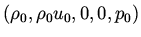 ,
,
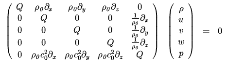 |
|
|
(63) |
in a domain
 ,
where
,
where
 (
(
 denotes the velocity vector),
with the solid wall boundary condition
denotes the velocity vector),
with the solid wall boundary condition
 |
|
|
(64) |
It is assumed that the problem was obtained by a linearization in a vicinity
of a boundary point, and that the far field boundary conditions were given
in terms of
characteristic variables, which are
not used explicitly in the derivation of the approximate Hessian.
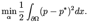
The minimization problem is
 |
|
|
(65) |
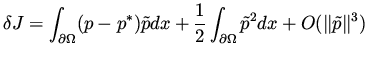
If a change  produces a change
  in the pressure then, the
variation in this functional can be written as
in the pressure then, the
variation in this functional can be written as
 |
|
|
(66) |
We calculate the Hessian in a slightly different way than before
to illustrate another approach.
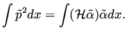
If one can express the quadratic term in in terms of
one can identify the Hessian.
That is,
 |
|
|
(67) |
This means that we can calculate the Hessian
without going through the adjoint variable.
We need to express in terms of , and
we do it in the Fourier space. From the boundary condition at the wall
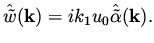 |
|
|
(68) |
The calculation of
 in terms of
 is done by
solving the system of the linearized Euler equation with the
above boundary condition for
is done by
solving the system of the linearized Euler equation with the
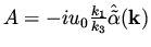
above boundary condition for  . We look for solution of the form
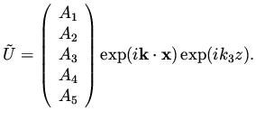 |
|
|
(69) |
The term  here is the analog of our
  in the previous example.
It is more convenient here due to the form of the symbol of the full
equation. The following relation follows by substituting the
above expression for
in the previous example.
It is more convenient here due to the form of the symbol of the full
equation. The following relation follows by substituting the
above expression for  into the Linearized Euler equations (63),
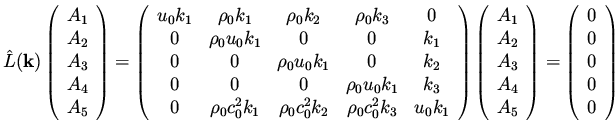 |
|
|
(70) |
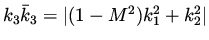
This is a linear system for
 and it has a nontrivial solution
when the determinant is zero,
and it has a nontrivial solution
when the determinant is zero,
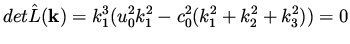 |
|
|
(71) |
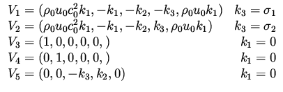
Note that there are five solutions for this equations. Each of them has a
corresponding solution for the vector
,
 |
|
|
(72) |
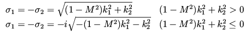
where
 |
|
|
(73) |
Note that for the subsonic case  correspond to the bounded solution,
while
correspond to the bounded solution,
while  to the unbounded one. When
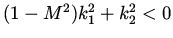 we have two bounded solution. In that case correspond to the incident
wave and therefore its amplitude is zero for the perturbation variables.
Thus, we are left with for both subsonic and supersonic cases.
The three solution corresponding to
we have two bounded solution. In that case correspond to the incident
wave and therefore its amplitude is zero for the perturbation variables.
Thus, we are left with for both subsonic and supersonic cases.
The three solution corresponding to  are not important for our analysis
since they do not affect the changes in pressure (see the corresponding
eigenvectors).
are not important for our analysis
since they do not affect the changes in pressure (see the corresponding
eigenvectors).
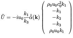
To summarize, only  contributes to the pressure changes as a
result of changes to the design variables by .
The solution for is given by
contributes to the pressure changes as a
result of changes to the design variables by .
The solution for is given by
 for some scalar
  . The
. The  component in this solution is
 and this must equal to
 form the boundary condition which in the Fourier space is given
by (68).
From that we find
form the boundary condition which in the Fourier space is given
by (68).
From that we find
 .
Thus the solution is,
.
Thus the solution is,
 |
|
|
(74) |
The last component in this vector gives us the change in the pressure
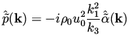 |
|
|
(75) |
and from this we get
 |
|
|
(76) |
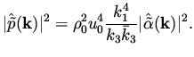
Notice that we have taken the complex conjugate of
, and
since  is a complex number its conjugate was taken as well.
Since
is a complex number its conjugate was taken as well.
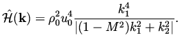
Since
 we obtain the symbol of the Hessian in the form,
 |
|
|
(77) |
A preconditioner for this problem is done exactly as in the small disturbance
equations using (60)-(62). It is also possible to construct the preconditioner
based on solution of the linearized Euler equations, but is more complicated
and unnecessary. The gradient  appearing in (60)-(62) has to be changed to the
gradient for this problem, using the adjoint formulation.
appearing in (60)-(62) has to be changed to the
gradient for this problem, using the adjoint formulation.
Next: Bibliography
Up: Application to Shape Design:
Previous: Three Dimensional Case
Shlomo Ta'asan
2001-08-22