


Next: The Linearized Euler Equations
Up: Small Disturbance Potential Equation
Previous: Two Dimensional Case
We distinguish here two cases,
the purely subsonic case and the general case which may include transonic
regimes.
Purely Subsonic Case.
In this case  and hence
 .
The preconditioner symbol is
.
The preconditioner symbol is
![$\displaystyle \hat {\cal R} ({\bf k}) = \left[ (1-M^2) k_1^2 + k_2^2 \right] / (\rho_0^2u_0 ^4 k_1^4).$](img139.png) |
|
|
(54) |
The preconditioned iteration will have in the Fourier space the direction
 |
|
|
(55) |
which after some rearrangements reads as
 |
|
|
(56) |
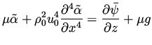
This equation in the Fourier space can be translated into the following
differential equation for the change in the design variable,
 |
|
|
(57) |
Actually, since our analysis was accurate only for the high frequency
changes, we may not want to use that preconditioning for the very
smooth components in the solution. This suggest a combination of the
standard gradient descent method and this preconditioning, which for example,
can be employed as
 |
|
|
(58) |
The addition of the  term is so that the low frequency range will not be
affected by this preconditioner and would just use the gradient direction.
High frequency on the other hand, are accurately analyzed by our method and
should use the above preconditioner.
It is also possible to use BFGS method in conjunction with
the infinite dimensional preconditioner developed here.
term is so that the low frequency range will not be
affected by this preconditioner and would just use the gradient direction.
High frequency on the other hand, are accurately analyzed by our method and
should use the above preconditioner.
It is also possible to use BFGS method in conjunction with
the infinite dimensional preconditioner developed here.
Supersonic and Transonic Cases.
In this case the term
 cannot be simplified and we have to treat a certain pseudo differential operator.
To approximate
we use the relation
cannot be simplified and we have to treat a certain pseudo differential operator.
To approximate
we use the relation
 |
|
|
(59) |
which was derived before, using the interior equations.
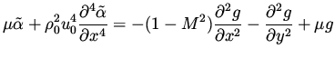
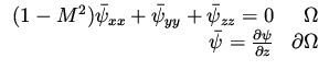
We want to derive an implementation in real space of the equation whose form in the
Fourier space is
The symbol
 represent two normal derivatives to solution
of the small disturbance equation we started with, one with the
represent two normal derivatives to solution
of the small disturbance equation we started with, one with the  equation and the other with the
  equation. The difference between the two is at the far field boundary condition which is responsible for the
proper choice in
equation. The difference between the two is at the far field boundary condition which is responsible for the
proper choice in
 .
The operator whose symbol is
is therefore constructed in two step.
.
The operator whose symbol is
is therefore constructed in two step.
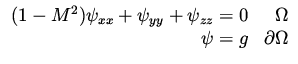 |
|
|
(60) |
 |
|
|
(61) |
and the full preconditioned direction for  is therefore
 |
|
|
(62) |
where
 satisfy the above equations.
Next: The Linearized Euler Equations
Up: Small Disturbance Potential Equation
Previous: Two Dimensional Case
Shlomo Ta'asan
2001-08-22