


Next: Application to Shape Design:
Up: The Main Idea
Previous: Constructing The Preconditioner from
The previous section discussed the construction of preconditioners from
their symbol in case the design space was a space of functions defined,
for example, on the boundary of a domain. This is the infinite dimensional
design space.
In many applications one uses a fixed
finite dimensional representation of the design space, using a set of
prescribed shape functions. When the number of these functions is small
one can use acceleration techniques such as BFGS. When that number grows and the number of BFGS
steps required to solve the problem increases significantly, one may combine a preconditioner which is based
on the infinite dimensional analysis.
We consider two design spaces. The first,  , is a space of functions
which is infinite dimensional and the second one,
, is a space of functions
which is infinite dimensional and the second one,  , is a subspace
of the first and is represented in terms of
, is a subspace
of the first and is represented in terms of  functions,
 .
We also assume that the set
is orthonormal with respect to
the usual
.
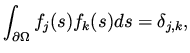
We also assume that the set
is orthonormal with respect to
the usual  inner product on the boundary,
 |
|
|
(27) |
where  is the Kronecker delta.
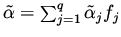
Functions in are linear combination of the form
is the Kronecker delta.
Functions in are linear combination of the form
 ,
and the space can be identified
,
and the space can be identified  . We construct
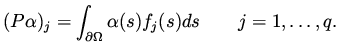
a mapping
. We construct
a mapping  from to by,
 |
|
|
(28) |
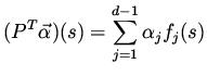
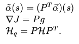
Note that the transpose of the operator acts from the finite dimensional
space to and is given by
 |
|
|
(29) |
where
 .
.
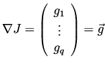
Now we come to the point of relating gradients calculated with respect to the
design space to those calculated with respect to .
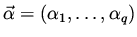
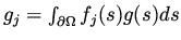
Let
 |
|
|
(30) |
be the variation of the functional corresponding to a change in the design
variables by
 . The gradient with respect to
is certainly
. The gradient with respect to
is certainly  , and the Hessian is
  .
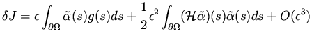
Now if the change in the design variables are done
in the subspace , we consider
.
Now if the change in the design variables are done
in the subspace , we consider
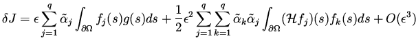
 and then
a substitution into the above expression for
and then
a substitution into the above expression for  gives
gives
 |
|
|
(31) |
and in that case
 |
|
|
(32) |
where
 ,
,
 , and the Hessian
for the subspace,
, and the Hessian
for the subspace,  , is related to the full Hessian as
 |
|
|
(33) |
Notice that for the finite dimensional design space we can write,
 |
|
|
(34) |
These are the abstract formulas for the discrete quantities for the
subspace as a function of the same quantities on the infinite dimensional
space.
A preconditioner for the finite dimensional design can be obtained by constructing
first the infinite dimensional preconditioner and then using the above formula
to get
 .
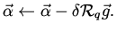
The preconditioned iteration is
.
The preconditioned iteration is
 |
|
|
(35) |
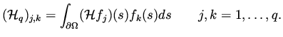
Example Consider the case
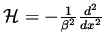 which appeared in one of the previous lectures.
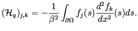
The finite dimensional preconditioner is constructed from the inverse of
the finite dimensional Hessian
which appeared in one of the previous lectures.
The finite dimensional preconditioner is constructed from the inverse of
the finite dimensional Hessian
 |
|
|
(36) |
Next: Application to Shape Design:
Up: The Main Idea
Previous: Constructing The Preconditioner from
Shlomo Ta'asan
2001-08-22