Next: Preconditioners for Finite Dimensional
Up: The Main Idea
Previous: The Main Idea
We come now to the question of constructing the preconditioner from its symbol.
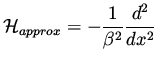
Since we are only interested in acceleration of
certain numerical procedure, it is enough to use approximations for the true
Hessians. Let us begin with the simplest examples.
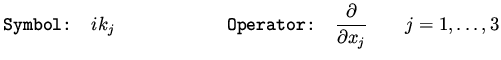
We have seen the correspondence between differential
operators and symbols,
 |
|
|
(9) |
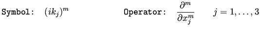
and therefore
 |
|
|
(10) |
Polynomials in  , even in several dimensions,
correspond to differential operators which are easily found as was shown in a previous
lecture.
, even in several dimensions,
correspond to differential operators which are easily found as was shown in a previous
lecture.
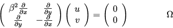
Example I. Consider the problem given in example V
in lecture no. 2.
subject to
with the boundary condition
where
 and
and
 .
It was shown there
that
.
It was shown there
that
 . This implies
that
. This implies
that
 |
|
|
(11) |
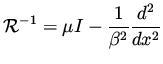
An effective
preconditioner  must satisfy
 for large
  and this is obtained for
 |
|
|
(12) |
The addition of the operator  was to ensure that the
preconditioner does not affect the low frequency range. A choice
was to ensure that the
preconditioner does not affect the low frequency range. A choice  can be
taken although some approximation of the first eigenvalue can give a better
choice.
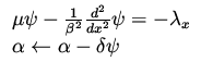
Thus, the implementation of a preconditioned iteration for that problem
consist of repeated application of the two steps
can be
taken although some approximation of the first eigenvalue can give a better
choice.
Thus, the implementation of a preconditioned iteration for that problem
consist of repeated application of the two steps
 |
|
|
(13) |
where  is found using a line search on coarse grids and,
  on
fine grids.
Note that the construction of the preconditioner was done on the differential
level but the numerical implementation is using some approximation of it, e.g.,
finite difference approximation.
on
fine grids.
Note that the construction of the preconditioner was done on the differential
level but the numerical implementation is using some approximation of it, e.g.,
finite difference approximation.
A good discretization (h-elliptic) of the state equation uses staggered grid.
We demonstrate it on a rectangular domain with a uniform grid of spacing  .
Let the grid points be labeled
.
Let the grid points be labeled
 .
The discrete variables approximating
.
The discrete variables approximating  will be located at the middle of the vertical
cell edges, i.e., will be parameterized as
will be located at the middle of the vertical
cell edges, i.e., will be parameterized as  . The discrete approximations to
 will be located at the middle of the horizontal edges, i.e., parameterized by
 . Discretization of the first equation is done at the cell centers
and the second equations at the vertices, both using central differences.
Design variables are located at the boundary nodes and the boundary
condition is given by
. Discretization of the first equation is done at the cell centers
and the second equations at the vertices, both using central differences.
Design variables are located at the boundary nodes and the boundary
condition is given by
 |
|
|
(14) |
A calculation of the cost functional for the discrete problem requires the
values of on the boundary  . This is done by introducing ghost variables
 . An extra equation for these ghost values is introduced at the
boundary nodes, approximating the second interior equation.
We introduce adjoint variables (Lagrange multipliers)
. An extra equation for these ghost values is introduced at the
boundary nodes, approximating the second interior equation.
We introduce adjoint variables (Lagrange multipliers)
 discretized as
 and
and  with ghost points
for
with ghost points
for  . The adjoint variables satisfy the same equation as
 but at points shifted by
  . A straightforward
calculation shows that the gradient is given by
. A straightforward
calculation shows that the gradient is given by
 |
|
|
(15) |
The discrete preconditioner is done as follows.
Let
 be the solution of the discrete problem
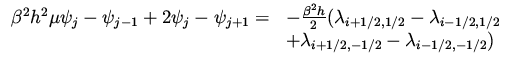 |
|
|
(16) |
for
 ,
where is the mesh size used for the discretization and
,
where is the mesh size used for the discretization and
 .
The design variables are updated by
.
The design variables are updated by
 |
|
|
(17) |
Note that applying the preconditioner requires the solution of a differential
equation on the boundary where the control is given. This is a typical case.
The equation defining the preconditioner is in one dimension less than
the state and the costate equations.
Example II.
We now move to a more challenging case which is the construction of an approximation
to a Hessian with a symbol
 , and the problem is on the boundary of a domain in three space dimensions.
Recall that in our lecture no 2 in this volume we have discussed the mapping
, and the problem is on the boundary of a domain in three space dimensions.
Recall that in our lecture no 2 in this volume we have discussed the mapping
 |
|
|
(18) |
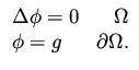
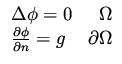
where  is the solution of a Laplace equation in the domain
 |
|
|
(19) |
and we have found that its symbol is
 |
|
|
(20) |
The construction of an operator  from functions defined on
the boundary of a domain, to functions defined on the same boundary,
whose symbol is
from functions defined on
the boundary of a domain, to functions defined on the same boundary,
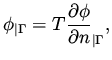
whose symbol is  is done as follows. Let
  be a function defined on the boundary of , we define
  by
by
 |
|
|
(21) |
where
 |
|
|
(22) |
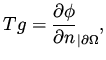
Another case we consider is an operator  whose symbol is
 |
|
|
(23) |
It can be approximated as
 |
|
|
(24) |
where
is the solution of
 |
|
|
(25) |
This follows from certain relations that we obtained in a previous lecture.
Example III. Here we
construct an operator whose symbol is
 .
We have a product of symbols, and each of them is something that we already
know. A product of symbols correspond to applying the corresponding operators one
after the other (with the proper order for systems of differential equations).
.
We have a product of symbols, and each of them is something that we already
know. A product of symbols correspond to applying the corresponding operators one
after the other (with the proper order for systems of differential equations).
The symbol
 correspond to the operator
 where
where  are the tangential coordinate corresponding to the wave directions
  respectively.
Let be the solution of (25)
then,
respectively.
Let be the solution of (25)
then,
 |
|
|
(26) |
has the desired symbol.
Remark:
The operators that we have constructed in the last example are nonlocal, and one may construct also integral operators
for them, with singular kernels. We prefer this approach since in the context of
the optimal design problems one already has a (fast) solver for the
equations needed for these pseudo-differential operators.
Next: Preconditioners for Finite Dimensional
Up: The Main Idea
Previous: The Main Idea
Shlomo Ta'asan
2001-08-22