


Next: Problem Reformulation
Up: Theoretical Tools for Problem
Previous: The Symbol of The
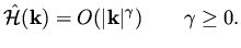
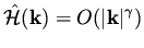
Using the symbol of the Hessian,
we can classify problems according to the
asymptotic behavior of
 for large
  .
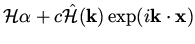
We consider the equation
.
We consider the equation
 |
|
|
(49) |
We want to classify problem into well-posed (good) problem, ill-posed (bad) problem,
easy problems and difficult problems.
Well posed problems are characterized by having a unique solution
that is stable to perturbation in the data of the problem.
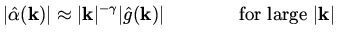
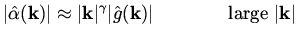
When we consider high frequencies, which is the range of frequencies
where our analysis of the Hessian is accurate, the following property
implies well posedness,
 |
|
|
(50) |
Note that a small
change in the design variable in the high frequency range
causes large changes in the right hand side, or the gradient.
Hence, small changes in the data results
in small changes in the solution, and the solution has the desired stability
properties.
This is summarized by
 |
|
|
(51) |
which follows from (35) and (50).
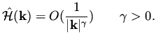
Ill-Posedness is referred to a case where
the solution is not unique or that it is sensitive to data in the problem.
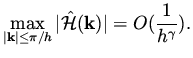
Ill-posedness that result from the behavior of high frequencies
can be characterized as
 |
|
|
(52) |
To see that such a behavior causes ill-posedness, consider a solution
 and a perturbation of it in the form
 .
The gradients evaluated for these two choices for the design variable
are
.
The gradients evaluated for these two choices for the design variable
are
 and
and
 . The latter can be approximated by
 |
|
|
(53) |
Since this is true for an arbitrary  and sufficiently large,
we get that
if is a solution then
is an approximate solution
for an arbitrary and sufficiency large . This implies that small
changes in the data of the problem will cause large changes in the solution.
It is summarized in the relation
and sufficiently large,
we get that
if is a solution then
is an approximate solution
for an arbitrary and sufficiency large . This implies that small
changes in the data of the problem will cause large changes in the solution.
It is summarized in the relation
 |
|
|
(54) |
which follows from (35) and (52),
which shows that small changes in the gradient are amplified significantly in
the design variables, for the high frequencies.
Thus, high frequencies in the design variables are unstable.
The Discrete Problem.
On a finite grid with mesh size  one consider
  in the range
 . Thus, for well-posed problems satisfying (50),
the eigenvalues of the Hessian corresponding
to the highest frequencies behave as
. Thus, for well-posed problems satisfying (50),
the eigenvalues of the Hessian corresponding
to the highest frequencies behave as
 |
|
|
(55) |
Since the smallest eigenvalue of the discrete Hessian is given approximately by
the corresponding eigenvalue of the differential Hessian,
the condition number of the Hessian behaves as
 .
This quantity is important in evaluating the performance of gradient based
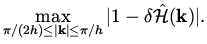
algorithms. As was mentioned in lecture 1, the convergence of gradient based
methods is determined by
.
This quantity is important in evaluating the performance of gradient based
algorithms. As was mentioned in lecture 1, the convergence of gradient based
methods is determined by
 , and the high frequency
components in the representation of the solution converge
at a rate
, and the high frequency
components in the representation of the solution converge
at a rate
 |
|
|
(56) |
The smallest eigenvalues of the Hessian are  being given approximately
by their values from the continuous problem.
From these observations we conclude that the expected rate of convergence for the full design problem is
therefore
being given approximately
by their values from the continuous problem.
From these observations we conclude that the expected rate of convergence for the full design problem is
therefore
 |
|
|
(57) |
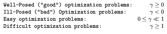
and that the complexity of a given problem can be
determined by the exponent  .
.
- Easy problems:
 .
.
- Difficult problems:

In summary, let the symbol of the Hessian satisfy
 |
|
|
(58) |
then, we have the following
 |
|
|
(59) |
Next: Problem Reformulation
Up: Theoretical Tools for Problem
Previous: The Symbol of The
Shlomo Ta'asan
2001-08-22