Problem Reformulation

Unlike the constraint PDE which governs the optimization problem under study, the parameter space as well as the cost functional are not uniquely determined for a given engineering task. It is very likely that a proper choice for one or both can lead to well posed problems that are easier to solve.

We demonstrate this fact by an example. The problem given in section 4.1 is shown to have good stability properties for the high frequencies. However, $\gamma=2$ for that problem, and the rate of convergence for gradient based methods is expected to be $1 - O(N^{-2})$ for $N$ design variables since $h = O( \frac{1}{N})$. Different choices for design space and cost functional will be shown to have a very different behavior, although the engineering task remains roughly the same.

Example VI: Design Variables Reformulation Consider the minimization problem

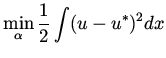$$\min_{\alpha} \frac{1}{2} \int (u - u^*)^2 dx$$ (60)

where $(u,v)$ satisfy the equations

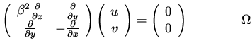$$\left( \begin{array}{cr} \beta^2 \frac{\partial }{\partial x}& \f... ...right)= \left( \begin{array}{c} 0 \\ 0 \end{array}\right) \qquad \qquad \Omega$$ (61)

with the boundary condition

$$v = \alpha \qquad \partial\Omega$$ (62)

where the domain $\Omega$ and $\beta$ are as before.

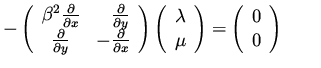
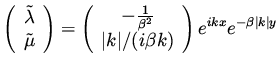
Following the same procedure as before, we introduce adjoint variables (Lagrange multipliers) $(\lambda, \mu)$ which can be shown to satisfy

$$- \left( \begin{array}{cr} \beta^2 \frac{\partial }{\partial x}& ... ...mu \end{array}\right)= \left( \begin{array}{c} 0 \\ 0 \end{array}\right)\qquad$$ (63)

with the boundary condition

$$-\mu + (u-u^*) = 0 \qquad \qquad \partial\Omega .$$ (64)

At the minimum the following equation has to be satisfied

$$- \lambda = 0 \qquad \qquad \partial \Omega,$$ (65)

and the gradient of the cost functional is given by

$$\nabla J = -\lambda _{\vert _{\partial\Omega}}.$$ (66)

Following a similar derivation as before we find that the perturbations $\tilde u, \tilde v, \tilde \lambda , \tilde \mu$ corresponding to a perturbation $\tilde \alpha = \exp (i k x )$ are

$$\left( \begin{array}{c} \tilde u \\ \tilde v \end{array}\right) ... ... \vert k \vert) \\ 1 \end{array}\right) e^{i k x}e^{ - \beta \vert k \vert y }$$ (67)

and

$$\left( \begin{array}{c} \tilde \lambda \\ \tilde \mu \end{array}... ...k \vert /(i \beta k) \end{array}\right) e^{ i k x} e^{- \beta \vert k \vert y }$$

Combining these results we obtain that the change in the gradient, corresponding to a change in the design variable by $\tilde \alpha = \exp (i k x )$ is

$${\cal H} \tilde \alpha = -\tilde \lambda _{\vert _{\partial\Omega}} = \frac{1}{\beta ^2} \exp (i k x)$$ (68)

Thus, the symbol of the Hessian is

$$\hat{\cal H} (k ) = \frac{1}{\beta ^2}$$ (69)

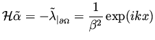
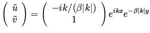
Remark. The boundary condition $v = \alpha _x$ correspond to a shape design problem where the shape is given by $\alpha (x)$, and the boundary condition there is $(u,v) \cdot {\bf n} =0$. As a result of the above calculation we can derive the following conclusion. If the design variables are the slopes instead of the shape itself, a well-posed problem is still obtained. Moreover, this problem is much easier to solve that the one for the shape directly. Note that from the engineering point of view both problems can be used to perform the required design. In the second one, a reconstruction of the shape from the slopes has to be done and this itself is a stable problem.