


Next: Fourier Analysis For Optimization
Up: On Pseudo-Differential Operators
Previous: On Pseudo-Differential Operators
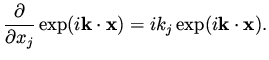
The operator  discussed above does not correspond to any differential operator.
Only polynomials in
discussed above does not correspond to any differential operator.
Only polynomials in  correspond to differential operators, and
this is via a very simple relation.
The differential operator
correspond to differential operators, and
this is via a very simple relation.
The differential operator
 corresponds to the symbol
  since
since
 |
|
|
(22) |
From this we have,
 |
|
|
(23) |
where
 and
and
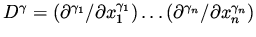 .
.
For a general operator , defined on functions in an infinite space,
we define the symbol
 by
by
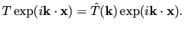 |
|
|
(24) |
This definition is for scalar PDE as well as for systems of PDE. In the
second case the symbol will be a matrix whose elements are functions of
.
A definition in a bounded domain  can also be done, by considering a small
vicinity of a point in and a localization of the above.
can also be done, by considering a small
vicinity of a point in and a localization of the above.
Using the definition (24) we see that we can define a larger class of operators by considering symbols which are not polynomials. Under some assumptions which we omit here, one gets the class of pseudo-differential operators.
They play a very important role in the study of boundary value problems for elliptic equations.
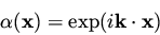
Example IV. We consider next the example
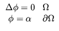 |
|
|
(25) |
where is any of the two domains in the previous example.
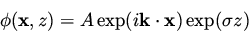
Following the same procedure as before,
 |
(26) |
 |
(27) |
implies
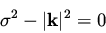 |
(28) |
and the relevant solution is
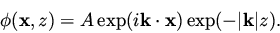 |
(29) |
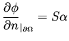
The value of  is determined from the boundary condition and
clearly we have
is determined from the boundary condition and
clearly we have
 |
|
|
(30) |
The relation of
 to the boundary values
 is described
by a mapping
is described
by a mapping 
 |
|
|
(31) |
whose symbol can be easily found by differentiating  in the outward
normal direction at the boundary, giving
in the outward
normal direction at the boundary, giving
 |
|
|
(32) |
Notice that although we are dealing with differential problems, some relation
between boundary values are not governed anymore by differential
operators.
The operators  from the last two examples
are therefore not differential operators but
pseudo-differential operators.
from the last two examples
are therefore not differential operators but
pseudo-differential operators.
Shape design problems are related to boundary control
problems, and therefore these type of operators play a very important role
in shape optimization. They will help us to characterize the minimization problem
in quantitative way that will allow the construction of very effective solvers.
Next: Fourier Analysis For Optimization
Up: On Pseudo-Differential Operators
Previous: On Pseudo-Differential Operators
Shlomo Ta'asan
2001-08-22