


Next: The Symbol of an
Up: Theoretical Tools for Problem
Previous: Review of Fourier Analysis
Fourier analysis can be used to understand more complicated questions.
For example, the relation of a function values to its normal derivative values
on the boundary. Some relations between the quantities of interest may
involve differential operators.
Other relations may involve a more general class of operators,
called pseudo-differential operators, which we briefly discuss here.
We consider elementary ideas from the theory of
pseudo-differential operators which we demonstrate using some simple
examples.
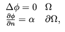
Example III Let  be the solution of the equation
 |
|
|
(13) |
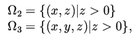
where the domain  is one of the two cases
 |
|
|
(14) |
and
 is the outward normal derivative at the
boundary.
is the outward normal derivative at the
boundary.
One of the questions we need to answer with regard to
shape optimization or boundary control problems is the nature of the mappings
between the control variable  , which in this case is a function defined
on the boundary, and say the value of the solution on the boundary.
That mapping is of course complicated and in general depends on the shape
of the domain . However, high frequencies in have only
local effect on the solution (this is a general property for elliptic
equations which we exploit ) and can be studied using Fourier techniques.
We take
, which in this case is a function defined
on the boundary, and say the value of the solution on the boundary.
That mapping is of course complicated and in general depends on the shape
of the domain . However, high frequencies in have only
local effect on the solution (this is a general property for elliptic
equations which we exploit ) and can be studied using Fourier techniques.
We take
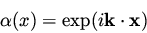 |
(15) |
where in case
 we take
 and
and
 , and for
 we take
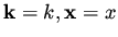 .
Then is given by
.
Then is given by
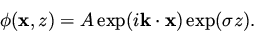 |
(16) |
A substitution of this expression for into the interior equation in (13)
implies
the following equation for 
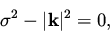 |
(17) |
and there are two solution
 |
(18) |
We look for a bounded solution in and
that is the one with
 .
The above expression for satisfies the interior equations in (13) for any
value of
.
The above expression for satisfies the interior equations in (13) for any
value of  , but
only one value will also satisfy the boundary condition.
Substituting (18) into that boundary condition, gives
, but
only one value will also satisfy the boundary condition.
Substituting (18) into that boundary condition, gives
 |
(19) |
The coefficient that we have just found gives a very important information.
It describes the mapping  between and the values of
on the boundary,
between and the values of
on the boundary,
 |
(20) |
What we have just found is a description of the mapping in
the Fourier space, i.e., the symbol of ,
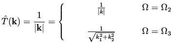 |
|
|
(21) |
A Remark: For a general domain
we consider a small vicinity of a boundary point
 ,
and if the boundary is smooth at that point, we can flatten this piece of boundary
by a proper transformation. We end up with a problem in half space,
of the same form as above. The relation between on the boundary, which is
flat now, and inside the domain can be easily calculated using
Fourier analysis.
,
and if the boundary is smooth at that point, we can flatten this piece of boundary
by a proper transformation. We end up with a problem in half space,
of the same form as above. The relation between on the boundary, which is
flat now, and inside the domain can be easily calculated using
Fourier analysis.
Subsections
Next: The Symbol of an
Up: Theoretical Tools for Problem
Previous: Review of Fourier Analysis
Shlomo Ta'asan
2001-08-22