


Next: On Pseudo-Differential Operators
Up: Theoretical Tools for Problem
Previous: Introduction
Fourier analysis has been a powerful tool for many years in analyzing
different numerical procedures, and it goes back to Von Neumann.
It can be used for a variety of tasks including
a quantitative information about the behavior of solutions, their dependence on
boundary values, etc. It can also be used to analyze numerical procedures
that we use to solve partial differential equations or optimization problems.
We go here briefly on the main ideas we need for the analysis of
optimization problems.
Let us begin by a simple problem, the linearized small disturbance potential
equation of
fluid dynamics. This equation will demonstrate the different issues we
are concerned with, and will set the foundation for the treatment of general
problems, including systems of equations such as the Euler and the Navier-Stokes equations.
Example I: A Scalar Equation.
Consider the equation
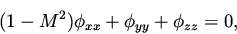 |
(1) |
in the domain
 .
This equation is an approximation for a flow in the x direction, where
perturbation velocities (around a mean velocity)
are related to the potential
.
This equation is an approximation for a flow in the x direction, where
perturbation velocities (around a mean velocity)
are related to the potential  as
as
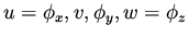 , see Hirsch [12].
We want to analyze the solution in terms of its
boundary values on  .
We consider boundary data in terms of Fourier components
.
We consider boundary data in terms of Fourier components
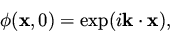 |
(2) |
where
 and
and
 .
We look for an exponential behavior in the
.
We look for an exponential behavior in the  direction
 |
(3) |
and a substitution of this expression
into equation (1) for leads to the relation
 |
(4) |
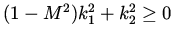
Note that this equation for  has two solutions. For
  one of them,
 , correspond to a
decaying solution for as a function of z and is considered as the solution of
interest. The other one,
, correspond to a
decaying solution for as a function of z and is considered as the solution of
interest. The other one,  , correspond to an unbounded solution
for
and is discarded.
Thus, for the subsonic case we have
, correspond to an unbounded solution
for
and is discarded.
Thus, for the subsonic case we have
 |
|
|
(5) |
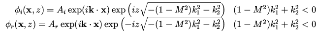
For the supersonic case,  , there are two bounded solutions for
 ,
and only one bounded solution for
,
and only one bounded solution for
 .
The two bounded solutions can be viewed as an
incident wave and a reflected wave,
whose sum satisfies the boundary condition,
.
The two bounded solutions can be viewed as an
incident wave and a reflected wave,
whose sum satisfies the boundary condition,
 |
|
|
(6) |
A general solution for the problem can be written as a sum (integral) of these
Fourier components.
Example II: A System of PDE. We next show the use of Fourier analysis for studying systems of partial differential equation. Consider the system
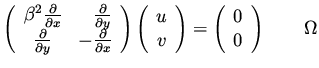 |
|
|
(7) |
where
 and
and
 .
Here one considers vector Fourier components, that is
.
Here one considers vector Fourier components, that is
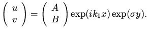 |
|
|
(8) |
The problem is to determine but also the relation of  and
and  .
This is done by substituting this form into the equations
leading to an algebraic equation for
.
This is done by substituting this form into the equations
leading to an algebraic equation for  ,
,
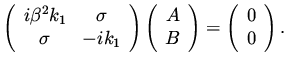 |
|
|
(9) |
This is a linear set of equations for the unknown and it has a non zero solution if and only if the determinant of the system is zero.
This gives an equation for in terms of  ,
,
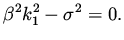 |
|
|
(10) |
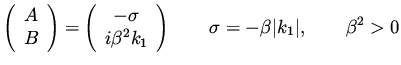
For the subsonic case  and we have only one solution
 , which correspond to a bounded solution in
  .
To find the relation of and we substitute
this value of into the system, and solve for yielding,
.
To find the relation of and we substitute
this value of into the system, and solve for yielding,
 |
|
|
(11) |
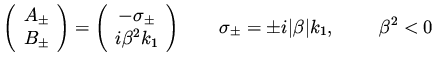
For the supersonic case,  , we have two solutions
 and
and
 corresponding to two bounded solution in , and the coefficients
are given by
corresponding to two bounded solution in , and the coefficients
are given by
 |
|
|
(12) |
The solution for given by (11) or (12) can be multiplied by an arbitrary
constant. The actual value of that constant depends on the boundary
condition which is required for the problem.
This complete the solution of the problem in .
Remark:
In general, there may be several solutions for and to each of them
there would correspond a vector solution such as
(11) or (12) in the example above. The general solution is then a
linear combination of these vectors with some weights to be determined from the
boundary conditions.
If the problem is well posed, then the number of boundary condition equals exactly
to the number of bounded solutions that we are seeking and the analysis
can be completed.
Some of the important question regarding general systems of equations can be
answered to some extent using this tool.
These include well-posedness of the problem, the choice of boundary conditions,
their effect on the solutions and more.
Next: On Pseudo-Differential Operators
Up: Theoretical Tools for Problem
Previous: Introduction
Shlomo Ta'asan
2001-08-22