Continuous Random Variables
Density functions
Definition 1. We say a random variable $X$ is continuous if there exists nonnegative integrable function $f_X$ such that $$ F_X(x) = \P( X \leq x) ) = \int_{-\infty}^x f_X(t) \, dt \,. $$ The function $f_X$ is called the density of $X$.
Remark 2. For arbitrary random variables, we recall the CDF is right continuous. If $X$ is a continuous random variable then $F_X$ is continuous, differentiable almost everywhere, and $F_X’ = f_X$.
Remark 3. You may be curious as to whether $F_X$ being continuous and / or differentiable almost everywhere implies the random variable $X$ is continuous. The answer (surprisingly) is no, and a counter example is given by this proposition.
Proposition 4. Let $X$ be a continuous random variable with with density $f_X$, then for every $a \in \R$, $\P(X = a) = 0$. Consequently, for any $[a, b] \subseteq \R$, $$ \P(X \in [a, b]) = \P(X \in (a, b)) = \int_a^b f_X(t) \, dt \,. $$
Standard distributions
Example 5 (Uniform distribution). We say $X \sim \Unif(a, b)$ if its density is given by $$ f_X(x) = \begin{cases} \displaystyle \frac{1}{b - a} & x \in [a, b] \\ 0 & \text{otherwise} \end{cases} $$
Recall the geometric distribution is memoryless. The analog of this for continuous random variables is the exponential distribution.
Example 6 (Exponential distribution). Let $\lambda > 0$ We say $X \sim \Exp(\lambda)$ if its density is given by $$ f_X(x) = \begin{cases} \displaystyle \lambda e^{-\lambda x} &x\geq 0 \,,\\ 0 & x <0 \,. \end{cases} $$
Problem 7. If $X$ is a continuous $[0, \infty)$-valued random variable. Show that $X \sim \Exp(\lambda)$ for some $\lambda > 0$ if and only if for every $s, t > 0$ we have the memoryless property $$ \P(X \geq s + t \given X \geq s) = \P( X \geq t ) \,. $$
Example 8 (Normal distribution). We say $X \sim \mathcal N(\mu, \sigma^2)$ if its density is given by $$ f_X(x) = \frac{1}{\sqrt{2\pi} \sigma} e^{\frac{-(x - \mu)^2}{2 \sigma^2}} $$
Remark 9. To check that the density of the normal distribution is a allowable density function, on needs to check that $\int_{-\infty}^\infty f_X(x) \, dx = 1$. This isn’t easy to do directly; however, if you assume $$ \int_{-\infty}^\infty e^{-x^2 / 2} \, dx = \sqrt{2\pi} \,, $$ then a change of variable easily verifies that for any $\mu, \sigma$, the normal density above integrates to $1$.
Problem 10. A “bad kicker” stands at the origin $(0, 0)$. He chooses $\theta \sim \Unif(-\pi/2, \pi/2)$, kicks the ball along the line that makes an angle $\theta$ with the positive $x$-axis. Say ball hits the line $y = 1$ at the point $(1, h)$. Find the density of $h$.
Answer. $h$ follows the standard Cauchy distribution
Expectations
So far we’ve only defined expectations of discrete random variables, but remarked that expectations of general random variables satisfy certain monotonicity conditions.
Proposition 11. If $X$ is a continuous random variable and the integral $$ \int_{-\infty}^\infty \abs{x} f_X(x) \, dx < \infty \,, $$ then $$ \E X = \int_{-\infty}^\infty x f_X(x) \, dx $$
Proof sketch. For convenience, we assume that for every $N$ the series $$ \sum_{k \in \N} \int_{k/N}^{(k+1)/N}\frac{k}{N} p(x) \, dx \quad\text{and}\quad \sum_{k \in \N} \int_{k/N}^{(k+1)/N}\frac{k+1}{N} p(x) \, dx $$ both converge absolutely for every $N \in \N$, and their limit (as $N \to \infty$) is exactly $\int_{-\infty}^\infty x f_X(x) \, dx$.
Set $X_N = \sum k \one_{k/N \leq X < (k+1) / N}$, $Y_N = \sum (k+1) \one_{k/N \leq X < (k+1) / N}$, and compare $\E X_N$, $\E X$, $\E Y_N$.
Theorem 12 (Lazy statistician). If $X$ is a continuous random variable, $g \colon \R \to \R$ is such that $g(X)$ is a continuous (or just a Borel) function, then $$ \E g(X) = \int_{-\infty}^\infty g(x) f_X(x) \, dx\,, $$ provided the integral converges absolutely.
Now the variance / standard deviation of continuous random variables can be computed
Proposition 13.
- If $X \sim \Unif(a, b)$ then $\E X = (a + b) / 2$ and $\var(X) = (b - a)^2 / 12$.
- If $X \sim \Exp(\lambda)$, then $\E X = 1 / \lambda$ and $\var(X) = 1 / \lambda$.
- If $X \sim \mathcal N(\mu, \sigma^2)$, then $\E X = \mu$ and $\var(X) = \sigma^2$.
Proposition 14 (Layer cake). If $X$ is a nonnegative continuous random variable for which $\E X$ is defined, then $$ \E X = \int_0^\infty \P(X \geq t) \, dt \,. $$
Remark 15. The layer cake formula holds for all nonnegative random variables for which $\E X$ is defined; however the tools we have so far only allow us to prove it in certain situations.
Proof sketch 1. Write $\E X$ as a double integral and Fubini.
Proof sketch 2. Compute $\E X$ by integrating by parts.
Multivariate distributions
Definition 16. Suppose $X_1, \dots, X_n$ are $n$ random variables, and let $X = (X_1, \dots, X_n)$.
- The joint distribution of $X_1$, …, $X_n$ is the probability measure on $\R^n$ defined by $$ \P_X(A) = \P(X \in A) \quad\text{for all Borel sets} A \subseteq \R^n \,. $$
- The joint cumulative density function is the function $F_X \colon \R^n \to [-1, 1]$ defined by $$ F_X(x_1, \dots, x_n) = \P( X_1 \leq x_1, \dots, X_n \leq x_n) $$
- We say $X = (X_1, \dots, X_n)$ is a continuous random vector if there exists a function $f_X \colon \R^n \to [0, \infty)$ such that for every $x = (x_1, \dots, x_n) \in \R^n$ we have $$ F_X(x_1, \dots, x_n) = \int_{-\infty}^{x_1} \cdots \int_{-\infty}^{x_n} f_X(x_1, \dots, x_n) \, dx_n \, \cdots \, dx_1 \,. $$ The function $f_X$ is called the joint density.
Proposition 17. The joint CDF $F_X$ always has the following properties:
- $F_X$ is increasing in each coordinate.
- Converges to $1$ as $(x_1, \dots, x_n)$ all approach $\infty$,
- Converges to and $0$ as $(x_1, \dots, x_n)$ all approach $-\infty$.
- Is right continuous in each coordinate.
Remark 18. If the random vector $X$ is continuous, then additionally:
- $F_X$ is continuous.
- The partials $\partial_i F_X$ exist almost everywhere and $\partial_i F_X = f_X$
Definition 19. Let $X = (X_1, \dots, X_n)$ be a random vector with joint distribution $\P_X$. The distribution of the $i$-th coordinate $X_i$ is called the $i$-th marginal of $\P_X$.
Proposition 20. If $F_X$ is the joint CDF of $X$, then the marginal CDFs are given by \begin{align} F_{X_1}(\textcolor{red}{x}) &= \lim_{x_2 \to \infty} \lim_{x_3 \to \infty} \cdots \lim_{x_n \to \infty} F_X(\textcolor{red}{x}, x_2, \dots, x_n) \\ F_{X_2}(\textcolor{red}{x}) &= \lim_{x_1 \to \infty} \lim_{x_3 \to \infty} \cdots \lim_{x_n \to \infty} F_X(x_1, \textcolor{red}{x}, x_3, \dots, x_n) \\ &\vdots \\ F_{X_n}(\textcolor{red}{x}) &= \lim_{x_1 \to \infty} \lim_{x_2 \to \infty} \cdots \lim_{x_{n-1} \to \infty} F_X(x_1, x_2, \dots, x_{n-1}, \textcolor{red}{x}) \end{align}
Proposition 21. Let $X = (X_1, \dots, X_n)$ be a continuous random vector, with joint density $f_X$. Then each $X_i$ is a continuous random variable, whose densities are given by \begin{align} f_{X_1}(\textcolor{red}{x}) &\defeq \int_{x_{2} = -\infty}^\infty \int_{x_3 = -\infty}^\infty \cdots \int_{x_n = -\infty}^\infty f_X(\textcolor{red}{x}, x_2, \cdots, x_n) \, dx_2 \, dx_3 \cdots \, dx_n \\ f_{X_2}(\textcolor{red}{x}) &\defeq \int_{x_{1} = -\infty}^\infty \int_{x_3 = -\infty}^\infty \cdots \int_{x_n = -\infty}^\infty f_X(x_1, \textcolor{red}{x}, \cdots, x_n) \, dx_1 \, dx_3 \cdots \, dx_n \\ &\vdots \\ f_{X_n}(\textcolor{red}{x}) &\defeq \int_{x_{1} = -\infty}^\infty \int_{x_2 = -\infty}^\infty \cdots \int_{x_{n-1} = -\infty}^\infty f_X(x_1, \cdots, x_{n-1}, \textcolor{red}{x} ) \, dx_1 \, dx_3 \cdots \, dx_{n-1} \end{align}
Remark 22. If each $X_i$ are continuous random variables, then $(X_1, \dots, X_n)$ need not be a continuous random vector.
Given the joint distribution $P_X$, you can recover the individual distributions as above. But given only the individual distributions, you can’t say anything about the joint distribution. Here are a few examples.
Problem 23. Let $X, X’, Z$ be independent variables such that $X$ and $X’$ have the same distribution, and $Z \sim \Bernoulli(p)$ for some $p \in [0, 1]$. Let $Y = ZX + (1 - Z) X’$. Let $F$ be the joint CDF of $X, Y$, and $F_1$, $F_2$ be the two marginals CDFs of $F$.
- Find $F_1$, $F_2$ in terms of $F_X$.
- Assuming $X$ has finite variance, find the Pearson’s correlation coefficient between $X$ and $Y$.
Problem 24. Let $f \colon \R \to (0, \infty)$ be a continuous PDF, and let $ F(x) = \int_{-\infty}^x f(t)\,dt $ be the corresponding CDF. Suppose $f$ is symmetric (i.e., suppose $f(-x)=f(x)$). Our aim is to construct several continuous joint distributions whose marginals are $f$.
Let $g \colon \R \to [0,\infty)$ be a continuous $1$-periodic function (i.e. $g(x+1)=g(x)$ for every $x\in\R$) such that $$ \int_0^1 g(t)\,dt=1. $$
Let $\alpha\in[0,1]$ and define $$ p_\alpha(u,v) \defeq \begin{cases} \alpha g(u-v)+(1-\alpha)g(u+v) & (u,v)\in[0,1]^2 \,, \\ 0 & \text{otherwise} \,. \end{cases} $$ Suppose $U_\alpha,V_\alpha$ are random variables with joint density $p_\alpha$.
- What are the marginal densities $f_{U_\alpha}$ and $f_{V_\alpha}$?
-
Let $F^{-1}\colon(0,1)\to\R$ be the inverse of $F$, and set $$ X_\alpha=F^{-1}(U_\alpha),\qquad Y_\alpha=F^{-1}(V_\alpha). $$ What are the marginal densities of $X_\alpha$ and $Y_\alpha$?
-
If $X_\alpha$, $Y_\alpha$ have finite variance, show that $$ \cov(X_\alpha,Y_\alpha) = \alpha\cov(X_1,Y_1) + (1-\alpha)\cov(X_0,Y_0). $$
Remark 25. By choosing $g(x) = \sum_{k \in \Z} \frac{1}{2\epsilon} \one_{-\epsilon, \epsilon}(x - k)$, and making $\epsilon$ small, one can make the Pearson’s correlation coefficient of $X_\alpha, Y_\alpha$ to be any prescribed value in $(-1, 1)$.
Proposition 26. Let $x, h \in \R^n$, and $A$ be the rectangle with opposite corners $x$ and $y$. Let $X$ be a continuous random vector with joint density $f_X$ Then $$\label{e:P}\tag{P} \P(X \in A) = \int_A f_X(x) \, dx = \int_{x_1}^{x_1 + h_1} \cdots \int_{x_n}^{x_n + h_n} f_X(x_1, \cdots, x_n) \, dx_1 \cdots dx_n \,. $$
Proof sketch when $n = 2$. \begin{align} \P( X \in (x_1, y_1] \times (x_2, y_2] ) &= F_X(y_1, y_2) - F_X(y_1, x_1) - (F_X(x_1, y_2) - F_X(x_1, x_2)) \\ &= \int_{x_1}^{y_1} \int_{x_2}^{y_2} f_X(x) \, dx \end{align} Now since each $X_i$ is a continuous random variable we get \eqref{e:P}.
Remark 27. Once \eqref{e:P} is true for rectangles $A$, one can show $$ \P(X \in A) = \int_A f_X(x) \, dx \,, $$ provided $A$ is nice enough for the integral on the right to be defined.
Theorem 28 (Lazy statistician). Let $X = (X_1, \dots, X_n)$ be a continuous random vector with (joint) density $f_X$. Let $g \colon \R^n \to \R$. Then $$ \E g(X) = \int_{\R^n} g(x) f_X(x) \, dx \quad\text{provided}\quad \int_{\R^n} \abs{g(x)} \, dx < \infty \,. $$
Remark 29. It’s no co-incidence that Theorem 28 looks like Theorem 12. The only difference is that in Theorem 28 the function $g$ has domain $\R^n$ and the integral is an $n$-dimensional (iterated) integral. In Theorem 12, however, the function $g$ has domain $\R$ and the integral is a one dimensional integral.
Problem 30. Let $R = [-1, 1]^2 \subseteq \R^2$ and define $$ f(x) = \one_{R}(x) \paren[\Big]{ 1 + \sum_{m,n = 1}^\infty a_{m, n} \sin(\pi m x_1) \sin(\pi x_2) } \,, $$ where $a_{m,n}$ are such that $\sum |a_{m, n}| < \infty$, and $f(x) \geq 0$ for all $x \in R$. Suppose $X = (X_1, X_2)$ is a 2-dimensional random vector with joint density $f$.
- Find the marginal densities of both $X_1$ and $X_2$.
- Find $\cov(X_1, X_2)$.
Independence
Recall for discrete random variables, $\set{X_n}_{n \in \N}$ are independent if for every $N \in \N$, $x_1, \dots, x_n \in \R$, $$\label{e:I1}\tag{I1} \P(X_1 = x_1, \dots, X_N = x_N) = \P(X_1 = x_1) \cdots \P(X_N = x_N) \,. $$ This doesn’t help for general random variables as the events $\set{X = x}$ may all have probability $0$. However, if we replace $\set{X = x}$ with $\set{X \leq x}$, we get what we need.
Definition 31. Let $\set{X_n}_{n \in \N}$ be a family of (not necessarily discrete) random variables. We say $\set{X_n}_{n \in \N}$ are independent if for every $N \in \N$ and every $x_1$, …, $x_N \in \R$, we have $$\label{e:I2}\tag{I2} \P(X_1 \leq x_1, \dots, X_N \leq x_N) = \P(X_1 \leq x_1) \cdots \P(X_N \leq x_N) \,. $$
Theorem 32. If $\set{X_n}_{n \in \N}$ is a family of independent random variables, then for sequence of Borel sets $A_1$, …, $A_N \subseteq \R$, the events $\set{ \set{X_n \in A_n} \st n \in \N}$ are independent.
Remark 33. Note for discrete random variables, for any $A \subseteq \R$, the event $\set{X \in A} \in \mathcal F$. This fails for random variables that are not discrete, and the event $\set{X \in A}$ is only guaranteed to be in $\mathcal F$ provided $A$ is nice (explicitly, provided $A$ is a Borel set). The proof of Theorem 32 in general requires some technicalities from measure theory which we will not cover. We will, however, mostly prove this for continuous random variables.
Proposition 34. Let $X_1$, …, $X_N$ be continuous random variables. Then $\set{X_1, \dots, X_n}$ are independent if and only if $X = (X_1, \dots, X_n)$ is a continuous random variable with density $$ f_X(x_1, \dots, x_n) = f_{X_1}(x_1) \cdots f_{X_n}(x_n) \,. $$
Corollary 35. If $\set{X_1, \dots, X_N}$ are continuous independent random variables, then for any collection of Borel sets $A_1$, …, $A_n$, the events $\set{X_1 \in A_1}$, …, $\set{X_n \in A_n}$ are independent and $$ \P(X_1 \in A_1, \dots, X_n \in A_n) = \P(X_1 \in A_1) \cdots \P(X_n \in A_n) \,. $$
Theorem 36. The sequence of random variables $\set{X_n}_{n \in \N}$ are independent if and only if for every $N \in \N$ and every bounded continuous functions $f_1$, …, $f_N \colon \R \to \R$ we have $$ \E \paren[\big]{ \prod_{n = 1}^N f_n(X_n) } = \prod_{n = 1}^N \paren[\big]{\E f_n(X_n)} \,. $$
Proof sketch. We already proved a more general version of this for discrete random variables. We don’t have the measure theory tools needed to prove this for general random variables; but we prove one direction for continuous random variables follows immediately from the lazy statistician formula.
Problem 37. For discrete random variables, prove that the new definition of independence is equivalent to the old one. That is prove \eqref{e:I1} holds for every $N \in \N$, $x_1$, …, $x_N \in \R$ if and only if \eqref{e:I2} holds for every $N \in \N$, $x_1$, …, $x_N \in \R$.
Note. Remember discrete random variables have a countable image; but not necessarily a discrete image. That is you can have discrete random variables that take on all rational values, for instance. In particular, given $x_1 \in X_1(\Omega)$, you can’t always find the “immediately preceding” value $x_1’ \in X_1(\Omega)$ (which you might be tempted to do as it makes the above problem simpler).
Theorem 38. If $X, Y$ are independent continuous random variables with densities $p$ and $q$ respectively, then $X + Y$ is a continuous random variable with density $p * q$. Here $p*q$ is the convolution of $p$ and $q$ defined by $$ p*q(x) = \int_{-\infty}^\infty p(x - y) q(y) \, dy = \int_{-\infty}^\infty p(y) q(x - y) \, dy \,. $$
Problem 39. Suppose $\set{X_n}_{n \in \N}$ are i.i.d. $\Unif(0, 1)$ distributed random variables. Let $S_N = \sum_{n = 1}^N X_n$, and $F_N$ be the CDF of $S_N$. Show that $$ F_N(x)=\frac1{n!} \sum_{k=0}^n (-1)^k \binom{n}{k} (x-k)_+^n \,. $$ (Here $y_{+} = \max\set{y, 0}$.)
Hint. There’s an elegant way to do this by inclusion / exclusion. Alternately, check $F_{N+1}(x) = \int_0^1 F_N(x - t) \, dt$ and prove this recursively.
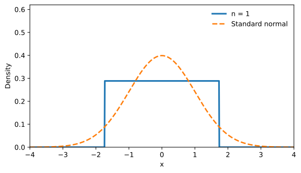
To foreshadow what’s to come, one natural question one could ask is whether there’s some interesting limiting behavior of $F_N$ as $N \to \infty$. If you look at the $f_N’s$ (the associated PDFs), center them, and rescale them (so they have variance $1$), they very quickly approach the PDF of the standard normal distribution!
Problem 40. If $X \sim \mathcal N(\mu, \sigma^2)$, and $Y \sim \mathcal N(\nu, \tau^2)$ are independent, find the distribution of $X + Y$.
Answer. $X + Y \sim \mathcal N(\mu + \nu, \sigma^2 + \tau^2)$.