The most challenging case is the infinite dimensional design case. It include all the possible difficulties one may encounter in an optimization problem. Our main goal here is to construct a relaxation that will smooth the design variables. That is, make high frequency changes in the design variables on fine grids, and low frequency changes on coarse grids. On each grid we want to update the design variables only in the scales that are high frequency for that level. In this way we split the design process on all levels of discretization. These ideas were developed by Arian and Ta'asan in [1],[2],[3].
In order to look for changes in the design variables we use the gradient, which is calculated using the adjoint method. Given an error in the design variables, one may ask the question how does the corresponding gradient look like. That is, suppose that our error is mainly a high frequency. Is it true or not that also the gradient will be dominated by high frequencies. The answer to this is given by the Hessian and we know how to analyze it using Fourier techniques as discussed in the previous lectures.
We consider example I of section 4.1. For the quasi-elliptic discretization
we know that no local relaxation (i.e., a relaxation based on the gradient)
can have the smoothing property, since the gradient does not 'feel'
the oscillatory parts in the errors of the design variables. Hence such errors
cannot be corrected efficiently by using the gradient.
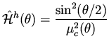
The h-elliptic discretization in that example had a symbol
![]() ,
and if we consider the expression
,
and if we consider the expression
| (47) |
| (48) |
In solving equations it is not so important to keep the low frequencies unchanged in the relaxation. It just gives the coarse levels an easier job. Here is it crucial not to introduce low frequency changes on the fine grids. The reason is that the corresponding effect on the state and costate has to be computed. When these changes are smooth this is not an inexpensive computation. Only the high frequency effect can be computed fast, due to the smoothing and to its localization to a vicinity of the boundary in elliptic problems.
In example II, the quasi-elliptic case does not have an efficient treatment,
as was in example I. The h-elliptic discretization in that example had a symbol
 |
(49) |
| (50) |
| (51) |
Preconditioners for Multigrid Relaxation.
To overcome difficulties such as in the last example,
we
introduce a preconditioner that is applied to the gradient
before using it to define a direction of change for the design variables.
Call that preconditioner ![]() , with a symbol
, with a symbol
![]() .
Our task is to choose
.
Our task is to choose
![]() such that
such that
 |
(52) |
The idea is to analyze the
behavior of
![]() and
and
![]() for the differential
problem, since in that case the computation is much simpler. This is followed by a discretization that does not violate h-ellipticity leading to a proper choice for
for the differential
problem, since in that case the computation is much simpler. This is followed by a discretization that does not violate h-ellipticity leading to a proper choice for
![]() .
.
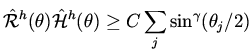
We therefore construct
![]() such that
such that
| (53) |
| (54) |
| (55) |
| (56) |
Notice that the relaxation does not requires a line search for the fine grids. The coarsest grids for which the analysis of the Hessian is not accurate enough uses a standard BFGS.
For example I of section 4.1 with the h-elliptic discretization
we obtain that the preconditioner ![]() should have a symbol
should have a symbol
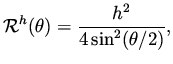 |
(57) |
 |
(58) |