


Next: Two Dimensional Case
Up: Application to Shape Design:
Previous: Application to Shape Design:
Let
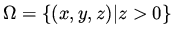 and let
  satisfy
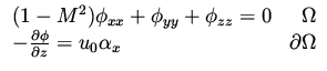 |
|
|
(37) |
and consider the minimization problem
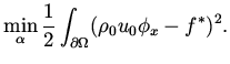 |
|
|
(38) |
This problem is related to a shape design problem governed by the Full Potential
equation in a general domain, using the cost functional
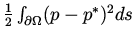 .
.
It can be shown using standard computation, as explained in a previous lecture,
that if  satisfies the
equation
satisfies the
equation
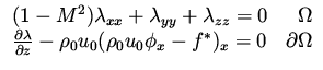 |
|
|
(39) |
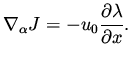
then the gradient of the functional is given by
 |
|
|
(40) |
We would like to compute the Hessian for this problem and to construct
an infinite dimensional preconditioner for it.
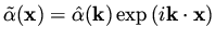
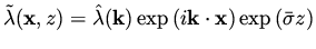
We assume a perturbation in  of the form
 |
|
|
(41) |
where
 and
and
 ,
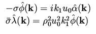
and then the corresponding change in is
,
and then the corresponding change in is
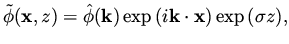 |
|
|
(42) |
and the change in the adjoint variable is
 |
|
|
(43) |
where
 are solutions for the following algebraic equation,
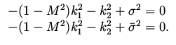 |
|
|
(44) |
In these expressions  are given, as well as
 which
amount to perturbing the shape by one frequency with a given amplitude.
which
amount to perturbing the shape by one frequency with a given amplitude.
The Choice of
. There is a nontrivial
point with respect to the choice of the roots that needs some explanation.
In the subsonic case,  , we have two real roots for
  . One is
negative
and correspond to a bounded solution in
. One is
negative
and correspond to a bounded solution in  , the other is
positive and correspond to an unbounded solution for
, the other is
positive and correspond to an unbounded solution for  and it
is discarded in our analysis.
In the supersonic case,
and it
is discarded in our analysis.
In the supersonic case,  , and the expression
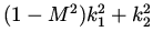 may be
either positive or negative. If it is positive we take for
the root mentioned above. If it is negative
then has two imaginary roots. One of these correspond to
an incident wave and the other to a reflected wave. The perturbation in
the incident wave is zero, since this wave comes from infinity and there
was no change there. The reflected wave arise from the change in shape.
In the supersonic regime, at the outflow there are no boundary conditions
for , while the adjoint
variable has two boundary conditions. Therefore,
for the perturbation in the adjoint variable
no waves are going toward the outflow. This means that the
sign of
may be
either positive or negative. If it is positive we take for
the root mentioned above. If it is negative
then has two imaginary roots. One of these correspond to
an incident wave and the other to a reflected wave. The perturbation in
the incident wave is zero, since this wave comes from infinity and there
was no change there. The reflected wave arise from the change in shape.
In the supersonic regime, at the outflow there are no boundary conditions
for , while the adjoint
variable has two boundary conditions. Therefore,
for the perturbation in the adjoint variable
no waves are going toward the outflow. This means that the
sign of  is opposite to that
of in the supersonic case
when wave solutions exist.
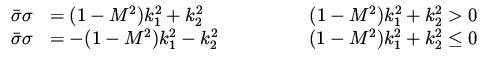
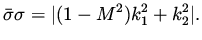
Therefore, the roots are
is opposite to that
of in the supersonic case
when wave solutions exist.
Therefore, the roots are
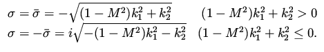 |
|
|
(45) |
From the boundary condition for and
we see that the following relations hold,
 |
|
|
(46) |
and from these the change in the gradient as a result of a change in
is given by
 and therefore,
 |
|
|
(47) |
Now notice that
 |
|
|
(48) |
and the two can be combined as
 |
|
|
(49) |
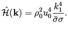
In summary, the symbol of the Hessian is
 |
|
|
(50) |
Subsections
Next: Two Dimensional Case
Up: Application to Shape Design:
Previous: Application to Shape Design:
Shlomo Ta'asan
2001-08-22