


Next: Constrained Optimization
Up: Review of The Basics:
Previous: Review of The Basics:
Consider the unconstrained minimization problem
 |
|
|
(1) |
where
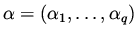 . We refer to
  as the
design variable and to
as the
design variable and to  as the cost functional.
A change in the design variables by
as the cost functional.
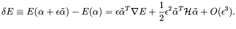
A change in the design variables by  introduces a change
in the functional which can be written as
introduces a change
in the functional which can be written as
 |
|
|
(2) |
Here
 and
and  stands for the Hessian, i.e., the matrix
of second derivatives of E.
We assume the Hessian is positive definite, i.e.,
stands for the Hessian, i.e., the matrix
of second derivatives of E.
We assume the Hessian is positive definite, i.e.,
 for all
  to guarantee a unique
minimum. For small
to guarantee a unique
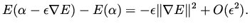
minimum. For small  we can neglect second order terms and higher in and see that a choice of
 result in a reduction of the functional, that is,
 |
|
|
(3) |
This is the basis for the steepest descent method and other
gradient based methods.
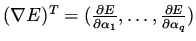
The gradient  of the functional
to be
minimized can be easily computed for this case, say, by finite
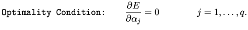
differences. At a minimum the following equations
hold,
of the functional
to be
minimized can be easily computed for this case, say, by finite
differences. At a minimum the following equations
hold,
 |
|
|
(4) |
These equations are called the (first order) necessary conditions for the problem.
Next: Constrained Optimization
Up: Review of The Basics:
Previous: Review of The Basics:
Shlomo Ta'asan
2001-08-22