


Next: Coarse Grid Optimization Problems
Up: One-Shot Multigrid Methods
Previous: One-Shot Multigrid Methods
In order to have a multigrid solver for the full optimization
problem with high efficiency, one has to guarantee that
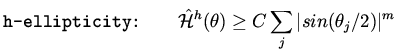
certain operators on the discrete level are h-elliptic.
In particular, the Hessian which is a symmetric positive definite
operator should have a discretization which is h-elliptic.
The Hessian may be a pseudo differential operator and its symbol may no longer be
a trigonometric polynomial. So we have to change slightly the definition of
h-ellipticity to include that case. Thus,
 |
|
|
(15) |
 |
|
|
(16) |
To demonstrate the difficulty that may arise with discretization we consider
the following example.
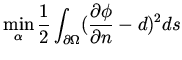
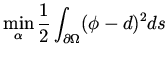
Example I: A Control Problem Let  be the state variable,
  the
design variable and consider the minimization problem,
the
design variable and consider the minimization problem,
 |
|
|
(17) |
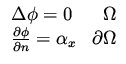
where satisfies
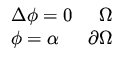 |
|
|
(18) |
and where
 .
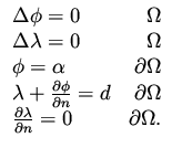
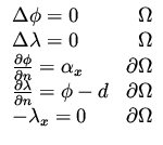
A simple calculation shows that the necessary (optimality) conditions are given by
.
A simple calculation shows that the necessary (optimality) conditions are given by
 |
|
|
(19) |
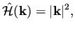
Following a calculation as in a previous lecture we obtain that the symbol
of the Hessian is given by
 |
|
|
(20) |
which is an elliptic symbol.
Consider now the following discretizations.
Discretization I: h-elliptic Hessian.
A uniform grid
with vertex discretization is used with the usual 5-point Laplacian
![$\displaystyle L^h = \frac{1}{h^2} \left[ \begin{array}{rrr} & 1 & \\
1 & -4 & 1 \\
& 1 & \end{array}\right].$](img38.png) |
|
|
(21) |
The discrete approximation to are parameterized as  where
where
 is a grid point.
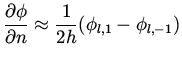
For discretization of the normal derivative at the boundary
we use a ghost point with a central discretization
is a grid point.
For discretization of the normal derivative at the boundary
we use a ghost point with a central discretization
 |
|
|
(22) |
where  stands for the boundary, and
  represent ghost points.
The above formula is used in discretization of the cost functional.
The actual implementation is to add one equation for the ghost point,
by approximating the interior equation also on the boundary. Thus,
relating the ghost values to other values in the interior.
represent ghost points.
The above formula is used in discretization of the cost functional.
The actual implementation is to add one equation for the ghost point,
by approximating the interior equation also on the boundary. Thus,
relating the ghost values to other values in the interior.
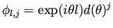
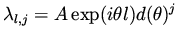
The design variables are taken at the grid vertices.
A Fourier change in by
 introduce the following changes
 |
|
|
(23) |
 |
|
|
(24) |
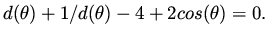
where
 is the solution of
 |
|
|
(25) |
Note that if  is a solution, then so is
 . The
first correspond to a bounded solution in half space while the other is unbounded.
Define
. The
first correspond to a bounded solution in half space while the other is unbounded.
Define
![$\displaystyle \mu (\theta ) = \frac{1}{2h} [ 1/d( \theta) - d ( \theta ) ]$](img51.png) |
|
|
(26) |
and observe that
 is
the symbol for normal derivative at the boundary.
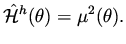
A simple calculation, as was done previously, shows that the symbol for the
discrete Hessian is
is
the symbol for normal derivative at the boundary.
A simple calculation, as was done previously, shows that the symbol for the
discrete Hessian is
 |
|
|
(27) |
To see that this is indeed h-elliptic notice that
 ,
and thus it is bounded away from zero.
,
and thus it is bounded away from zero.
Discretization II: Quasi-elliptic Hessian.
Here we consider a cell-centered scheme, i.e., the variables
approximating are located at the center of the cells and the control
variables  are located at the boundary grid points. The discretization
for the interior points is the same as before. The boundary condition also
here uses ghost points with a central discretization for Neumann boundary condition.
If we denote the grid points by then the variable are
are located at the boundary grid points. The discretization
for the interior points is the same as before. The boundary condition also
here uses ghost points with a central discretization for Neumann boundary condition.
If we denote the grid points by then the variable are
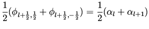
 The contribution of to the boundary condition at a general point
in the bottom boundary is
The contribution of to the boundary condition at a general point
in the bottom boundary is
 |
|
|
(28) |
where are the boundary points and
 are the ghost variables.
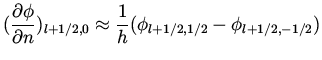
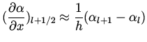
The Neumann derivative is approximated by
are the ghost variables.
The Neumann derivative is approximated by
 |
|
|
(29) |
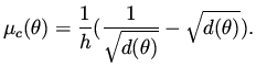
and the corresponding symbol is
 |
|
|
(30) |
Defining
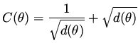 |
|
|
(31) |
the solution is given by
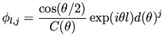 |
|
|
(32) |
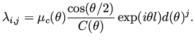 |
|
|
(33) |
Again a simple calculation shows that
symbol of the Hessian is
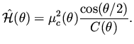 |
|
|
(34) |
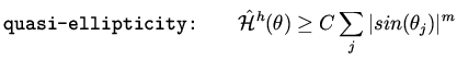
Since
 vanishes at
  the symbol is not h-elliptic, but only
quasi-elliptic. This means that no local relaxation of the design variables
will result in smoothing. That is, high frequency errors in the design
variable will not be damped fast. A standard multigrid method will not work
for this discretization.
In this example one could guess the quasi-ellipticity of the Hessian from the fact that
perturbation in the design variable of the form
the symbol is not h-elliptic, but only
quasi-elliptic. This means that no local relaxation of the design variables
will result in smoothing. That is, high frequency errors in the design
variable will not be damped fast. A standard multigrid method will not work
for this discretization.
In this example one could guess the quasi-ellipticity of the Hessian from the fact that
perturbation in the design variable of the form  do not cause any
changes in .
do not cause any
changes in .
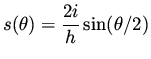
Example II:
Consider the optimization problem
 |
|
|
(35) |
 |
|
|
(36) |
subject to the equation,
 |
|
|
(37) |
where
.
A simple calculation shown that the necessary conditions are given by
 |
|
|
(38) |
and the symbol of the Hessian is
 |
|
|
(39) |
Discretization I: h-elliptic Hessian.
We use here cell-centered discretization for the state and costate and the
design variables are at the boundary nodes. The approximation
for the tangential derivative is
 |
|
|
(40) |
whose symbol is given by
 |
|
|
(41) |
The normal derivative is the same as in discretization II of example I.
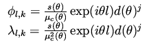
A change in the design variable by a Fourier component
results in the following
changes in state and costate
 |
|
|
(42) |
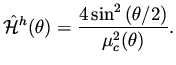
and the symbol of the Hessian is
 |
|
|
(43) |
We gave this example to show that although the symbol of the Hessian for the
differential
level was just the constant 1, on the discrete level the Hessian is more
complicated. Taylor expansion of this symbol at  shows that
it indeed approximate the PDE. Note however, that the Hessian has a
condition number which is independent of h. The ratio of largest to smallest
value that the symbol attains is independent of
shows that
it indeed approximate the PDE. Note however, that the Hessian has a
condition number which is independent of h. The ratio of largest to smallest
value that the symbol attains is independent of  .
This means that this problem presents no special difficulties even for very
large number of design variables.
.
This means that this problem presents no special difficulties even for very
large number of design variables.
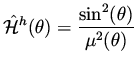
Discretization II: Quasi-elliptic Hessian.
Here we discretized the problem using cell-vertex variables for the
state and adjoint variables. The
design variables are given at the boundary nodes.
A simple calculation shows that
 |
|
|
(44) |
and this is a quasi-elliptic symbol, due to the
 term,
which vanishes at
term,
which vanishes at  .
.
Next: Coarse Grid Optimization Problems
Up: One-Shot Multigrid Methods
Previous: One-Shot Multigrid Methods
Shlomo Ta'asan
2001-08-22