next up previous
Next: Relaxation Up: One-Shot Multigrid Methods Previous: Discretization Issues

Coarse Grid Optimization Problems

Having discussed the main issues regarding discretization and h-ellipticity for optimization problems we move to the next major issue. The formulation of appropriate coarse grid equation that will serve to accelerate the fine grid optimization problem. We show that it is necessary in general to work with the adjoint variables (Lagrange multipliers) in order to define a proper coarse grid problem.

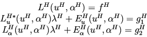
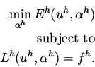
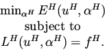
Consider the minimization problem

\begin{eqnarray*}
\min_{\alpha ^h} E^h(u ^h, \alpha ^h) \\
\mbox{\rm subject to} \\
L^h(u^h, \alpha ^h) = f^h.
\end{eqnarray*}


At the minimum the following equation holds (see the first lecture)

\begin{eqnarray*}
\begin{array}{c}
L^h(u^h, \alpha ^h) = f^h \\
L_u^{h*} (u^h,...
...^h \ (u^h, \alpha ^h) \lambda ^h + E_{\alpha}^h = 0.
\end{array}\end{eqnarray*}


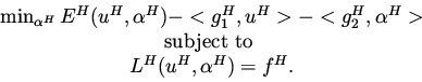
Next consider an attempt to define a coarse grid minimization problem that will accelerate the convergence of the fine grid above. We will show that without the use of Lagrange multipliers this is in general impossible. An argument for a quadratic functional and linear constraint is given in Ta'asan [7]. Consider the coarse grid minimization problem

\begin{eqnarray*}
\begin{array}{c}
\min_{\alpha ^H} E^H(u ^H, \alpha ^H) \\
\mbox{\rm subject to} \\
L^H(u^H, \alpha ^H) = f^H.
\end{array}\end{eqnarray*}


The necessary conditions for this problem are

\begin{eqnarray*}
L^H(u^H, \alpha ^H) = f^H \\
L_u^{H*}(u^H, \alpha ^H) \lambda...
...(u^H, \alpha ^H) \lambda ^H + E_{\alpha}^H (u^H, \alpha ^H) = 0.
\end{eqnarray*}


In order for this coarse grid equation to accelerate the fine grid solution process we must have the property that if the fine grid equations are solved, the coarse grid will not introduce any change to the fine grid solution. 
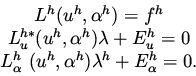
This means that the coarse grid function $I_h^H u^h , \bar{I}_h^H \alpha ^h $ must satisfy the coarse grid equation (Recall that the interpolation step is using the correction $u^H - I_h^H u^h, \alpha ^H - \bar I_h^H \alpha ^h $). From the first equation we see that we must have $f^H = L^H (I_h^H u^h, \bar{I}_h^H \alpha ^h) $, and from the second and third coarse grid necessary condition we see that there must exists a function $\lambda ^H$ that satisfies simultaneously the two equation $L_u^{H*}(I_h^H u^h, \bar{I}_h^H \alpha ^h) \lambda ^H = - E^H_u (I_h^H u^h, \bar{I}_h^H \alpha ^h) $ and $L_{\alpha}^H(I_h^H u^h, \bar{I}_h^H \alpha ^h) \lambda ^H = - E_{\alpha}^H (I_h^H u^h, \bar{I}_h^H \alpha ^h) $. But since the the two right hand sides are independent, in general, we have twice the number of equations than the number of unknowns in $\lambda ^H$. Thus, in general $I_h^H u^h , \bar{I}_h^H \alpha ^h $ will not be the solution of the coarse grid minimization problem.

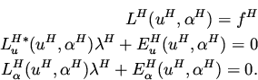
The correct way to define the coarse grid minimization problem is to start with the FAS equations for the necessary conditions. Thus, we get

\begin{eqnarray*}
\begin{array}{c}
L^H(u^H, \alpha ^H)= f^H\\
L_u^{H*}(u^H, \al...
...)\lambda ^H + E_{\alpha}^H (u^H,\alpha ^H)= g_2^H \\
\end{array}\end{eqnarray*}


where $f^H, g_1^H, g_2^H$ are the FAS transfers of the necessary conditions. The corresponding minimization problem whose necessary conditions are the above equation is the proper choice for the coarse grid optimization problem. This leads to the following coarse grid optimization problem

\begin{eqnarray*}
\begin{array}{c}
\min_{\alpha ^H} E^H( u^H, \alpha ^H) - <g_1^...
...\mbox{\rm subject to } \\
L^H(u^H, \alpha ^H) = f^H.
\end{array}\end{eqnarray*}


Note that in this formulation the functional has two extra terms $g_1^H,g_2^H$ which depend on the fine grid adjoint variables (Lagrange multipliers) through the FAS transfers for $g_1^H,g_2^H$.


next up previous
Next: Relaxation Up: One-Shot Multigrid Methods Previous: Discretization Issues
Shlomo Ta'asan 2001-08-22