


Next: Shape Design Problems
Up: Introduction to Shape Design
Previous: Quasi-Newton Methods
Shape optimization problems which are one of our main topics,
are related to control problems governed by PDE. An understanding
of boundary control problems will help us to get the proper insight
into shape optimization problems.
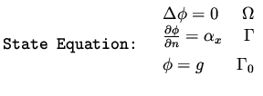
We consider the small disturbance equation, for zero Mach number,
in two dimensions. The domain  is a rectangle
whose bottom boundary has a control variable to be optimized.
It is required to achieve a certain pressure distribution on that boundary.
Denote by
is a rectangle
whose bottom boundary has a control variable to be optimized.
It is required to achieve a certain pressure distribution on that boundary.
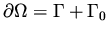
Denote by  the bottom boundary and by
  the rest of the
boundary . The potential
the rest of the
boundary . The potential  satisfies the equation
 |
|
|
(30) |
where  is the design variable.
This problem is related to a shape design problem in which the bottom
boundary is described by the function , and the boundary condition
for on this boundary is
is the design variable.
This problem is related to a shape design problem in which the bottom
boundary is described by the function , and the boundary condition
for on this boundary is
 . We will come to this relation
later on.
. We will come to this relation
later on.
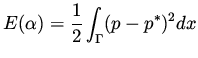
We consider the cost functional
 |
|
|
(31) |
where  ,
and we would like to construct a formula for the gradient of this functional.
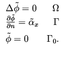
We consider a perturbation of the design variable by
,
and we would like to construct a formula for the gradient of this functional.
We consider a perturbation of the design variable by
 and the corresponding change in by
 , which
satisfies
, which
satisfies
 |
|
|
(32) |
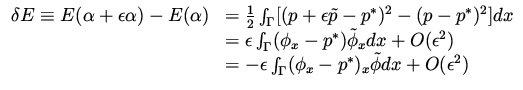
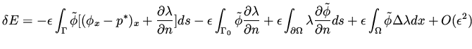
The variation in the functional is
 |
|
|
(33) |
where integration by parts have been used in the last equality.
As in the abstract constrained optimization problem we discussed in
section (2.2),
we see that the change in the functional depends on the the sensitivity
derivatives  , and we would like to eliminate this dependence,
in order to get an efficient computation of the gradient.
We do it by adding a term to
, and we would like to eliminate this dependence,
in order to get an efficient computation of the gradient.
We do it by adding a term to  which is the differential analog
of the term
which is the differential analog
of the term
 in the algebraic case. Then a proper choice for
  will result in the
desired form for the variation in the functional.
will result in the
desired form for the variation in the functional.
Let be an arbitrary function defined in the same domain as .
From equation (32) for we have
 |
|
|
(34) |
where the second equality follows from integration by parts.
This is the analog of equation (10) that we have in the algebraic case.
Adding the right hand side of (34) (multiplied by  ) to we get
 |
|
|
(35) |
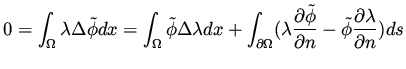
Since
 we can break the integral
 into
into
 and then combine the
  terms, to obtain
 |
|
|
(36) |
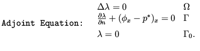
In order to eliminate the dependence of on
we make the following choice for
 |
|
|
(37) |
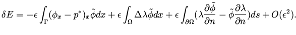
Therefore,
 |
|
|
(38) |
where integration by parts was used in the last equality.
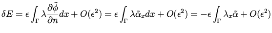
The expression for the changes in the functional is given
as as a function of the changes in the
design variable, as well the adjoint variable which satisfies
the adjoint equation (37),
(or costate equation in control terminology).
We would like now to pick a direction of change  that will
result in reduction of the cost functional. We distinguish two cases.
that will
result in reduction of the cost functional. We distinguish two cases.
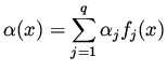
I. Finite Dimensional Control. In this case we assume that the
design variable  has a representation
 |
|
|
(39) |
and a similar expression for , where the functions
 are prescribed.
This implies
are prescribed.
This implies
 |
|
|
(40) |
and hence
 |
|
|
(41) |
and the choice
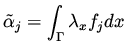 |
|
|
(42) |
will result in a reduction of the cost functional by
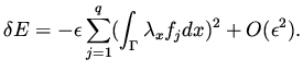 |
|
|
(43) |
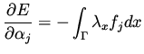
At a minimum the following conditions hold,
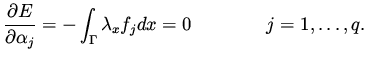 |
|
|
(44) |
Note that the gradient given in (44) is in terms of .
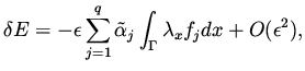
II. Infinite Dimensional Control. In this case we regard the variable
as a function defined on the boundary . A proper choice that will
result in a reduction of the functional is given in terms of ,
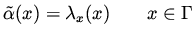 |
|
|
(45) |
and the corresponding reduction in the functional
is given this time by
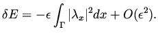 |
|
|
(46) |
An algorithm for solving this control
problem consists of repeated application of the following three steps,
until convergence (of the gradient to zero),
ALGORITHM
(1) Solve the state equation (30) for
(2) Solve the adjoint equation (37) for
(3) Update by
 , where
  is found by line search.
 is given by (42) or (45).
Next: Shape Design Problems
Up: Introduction to Shape Design
Previous: Quasi-Newton Methods
Shlomo Ta'asan
2001-08-22