


Next: Shape Design Using The
Up: Applications to Fluid Dynamics
Previous: Applications to Fluid Dynamics
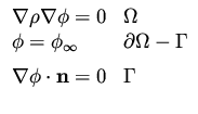
Consider the Full Potential (FP) equation
 |
|
|
(63) |
where  with
with
 and the following
shape optimization problem,
and the following
shape optimization problem,
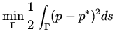 |
|
|
(64) |
where  .
We derive the necessary conditions for this problem, and obtain a formula for
the gradient for this functional subject to the FP equation (63).
.
We derive the necessary conditions for this problem, and obtain a formula for
the gradient for this functional subject to the FP equation (63).
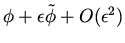
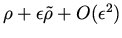
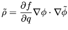
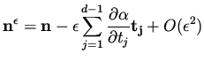
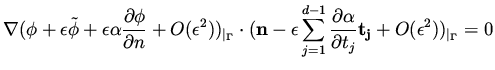
As a result of changes in the shape  , the potential changes to
 and
and  into
into
 .
Moreover,
.
Moreover,
 |
|
|
(65) |
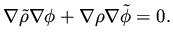
and
the equation governing  is
is
 |
|
|
(66) |
The functional variation with respect to
(see equation (62)) can be written as
![$\displaystyle \delta J
= \epsilon \int _{\Gamma} (p - p^*) \tilde p ds + \epsil...
...c{\partial p}{\partial n}(p-p^*) - \frac{(p-p^*)^2}{2R} ] ds + O( \epsilon ^2).$](img164.png) |
|
|
(67) |
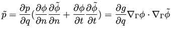
From the boundary condition
 some terms are simplified, in particular
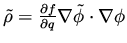
![$\frac{\partial p}{\partial n}= \frac{1}{2} \frac{\partial g}{\partial q}\frac{\...
...{\partial n}) ^2 + \sum_{j=1}^{d-1} (\frac{\partial \phi}{\partial t_j})^2] = 0$](img165.png) .
We also have the relation
.
We also have the relation
 |
|
|
(68) |
where
 stands for the tangential gradient.
Substituting these into
stands for the tangential gradient.
Substituting these into  and
using integration by parts for the
and
using integration by parts for the
 terms gives
![$\displaystyle \delta J = - \int _\Gamma [ \tilde \phi \sum _{j=1}^{d-1} \frac{\...
...) \frac{\partial \phi}{\partial t_j}\right) + \alpha \frac{ (p-p^*)^2}{2R} ] ds$](img170.png) |
|
|
(69) |
This expression depends on which is to be eliminated using the same
idea as before. To this end
we use the identity
 |
|
|
(70) |
which follows from (66) and holds for an arbitrary  .
The relation
.
The relation
 and
integration by parts of each of the terms in the above integral give
and
integration by parts of each of the terms in the above integral give
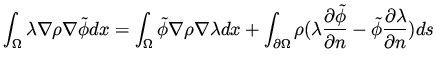
![$\displaystyle \int _\Omega \lambda \nabla \frac{\partial f}{\partial q}[\nabla ...
...\frac{\partial f}{\partial q}[\nabla \lambda \cdot \nabla \phi ] \nabla \phi dx$](img173.png) |
|
|
(71) |
 |
|
|
(72) |
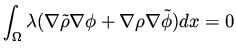
where in the first integral we used the relation
 on
as well as
on
as well as
 and
and
 on
on
 .
Thus,
.
Thus,
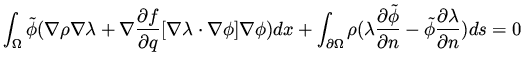 |
|
|
(73) |
for an arbitrary smooth function . This is the analog of equation (10)
of section (2.2).
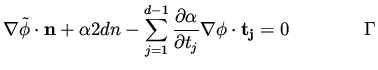
Before we add this term to the functional we need to express certain
terms in the boundary.
The wall boundary condition for  on
on

 |
|
|
(74) |
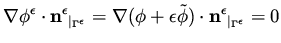
will be transfered to .
It is easy to see that
 |
|
|
(75) |
by considering one dimension at a time.
Therefore
 |
|
|
(76) |
Using the boundary condition
 we
get
we
get
 |
|
|
(77) |
The expression for the change in the functional as given in (69)
depends on  as
well as on . To eliminate the dependence on we add
the left hand side of (73).
We then collect terms involving separately from
terms involving
as
well as on . To eliminate the dependence on we add
the left hand side of (73).
We then collect terms involving separately from
terms involving
 , and use the boundary condition for
on , giving
, and use the boundary condition for
on , giving
![$\displaystyle \begin{array}{ll}
\delta J = & -\int _\Gamma \tilde \phi [\sum _{...
... f}{\partial q}[\nabla \lambda \cdot \nabla \phi ] \nabla \phi ) dx
\end{array}$](img186.png) |
|
|
(78) |
Now we choose such that it satisfies
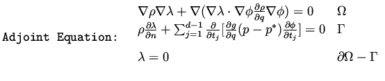 |
|
|
(79) |
and then the variation of the functional simplifies to
![$\displaystyle \delta J = - \int _\Gamma \alpha [ \rho \lambda \dphi2dn + \frac{...
...partial}{\partial t_j} ( \lambda \rho \frac{\partial \phi}{\partial t_j}) ] ds.$](img188.png) |
|
|
(80) |
The gradient of the functional is given by
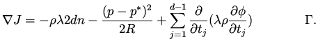 |
|
|
(81) |
Next: Shape Design Using The
Up: Applications to Fluid Dynamics
Previous: Applications to Fluid Dynamics
Shlomo Ta'asan
2001-08-22