Consider the following rational function g which is a straight line with a hole in it at x=-1.

> g:=x->(x^2-x-2)/(x+1);

To calculate the limit of g as x approaches -1, we first get MAPLE to typeset the limit so that we can see that

we are asking the limit that we want. Then we ask MAPLE to evaluate it by typing value(%) which means "find the value of the previous expression"

> Limit(g(x),x=-1);value(%);

One can also do left and right hand limits with MAPLE:

> g:=x->(x-8)/abs(x-8);

> plot(g(x),x=0..16);

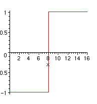
To get rid of the misleading vertical line in this plot we use the plot-option "style=point":

> plot(g(x),x=0..16,style=point);

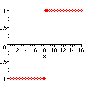
One does left and right hand limits simply by using the additional optional argument to Limit, "left" or "right".

> Limit(g(x),x=8,left);value(%);

> Limit(g(x),x=8,right);value(%);

When the left and right hand limits are not the same then of course the limit does not exist and so MAPLE says that it is undefined.

> limit(g(x),x=8);

Here is the famous limit which is classically proved using the "Squeeze Theorem".

> h:=x->sin(x)/x;

> limit(h(x),x=0);

Sometimes MAPLE neither gives you the value of the limit nor does it declare that the limit is undefined but it

does provide useful information.

> k:=x->sin(1/x);

> plot(k(x),x=-1..1);

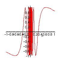
You can see from the graph that the y-value does not approach any particular value but it oscillates between +1 and -1 infinitely often. MAPLE kinda says this:

> Limit(k(x),x=0);

> limit(k(x),x=0);

Suppose that you throw a ball up in the air on the moon. The distance travelled after t seconds is given by:

> s:=t->58*t-0.83*t^2;

To calculate the instantaneous velocity of the ball at t=5 seconds, we can calculate the average rate of change over small intervals near t=5 and let these intervals shrink in length and observe their limiting behavior. The average rate of change is a called a "difference quotient":

> diffq:=h->(s(5+h)-s(5))/h;

We can now let the length of the interval get very small...

> diffq(1);

> diffq(0.5);

> diffq(0.1);

> diffq(0.0001);

Piecewise defined functions are easily entered into MAPLE. First enter it as an expression so that you can check that you have typed what you want:

> p:=piecewise(x<5,-x^2,x>5,3*x-4);

Next enter it as a function so that it is easy to work with:

> p:=x->piecewise(x<5,-x^2,x>5,3*x-4);

Let's test the function with a few points in either side of the "cut-point" x=5:

> p(2);

> p(7);

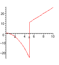
Note that if you plot the function, you get the misleading vertical line which you can get rid of with "style=plot" as discussed above.

> plot(p(x),x=0..10);

> plot(p(x),x=0..10,style=point);

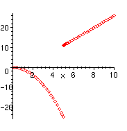
Let's calculate the limit of p:

> Limit(p(x),x=5);value(%);

As is obvious from the graph, the left and right hand limits do exist although they are not equal:

> limit(p(x),x=5,left);

> limit(p(x),x=5,right);

In the following limit, to get the exact answer, one could first "conjugate" and then multiply top and bottom of the result by 1/x. On the denominator express 1/x as 1/sqrt(x^2).

> k:=x->sqrt(3*x^2+8*x+6)-sqrt(3*x^2+3*x+1);

Let's first plug in a large value for x. Of course this proves nothing but it is a good thing to do:

> evalf(k(1000));

Let's see if a graph suggests that the limit is near this number:

> plot(k(x),x=0..100,y=1..2);

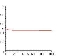
MAPLE will give the exact answer. Note the infinite limits are done using "infinity":

> Limit(k(x),x=infinity);value(%);

> evalf(%);

Next consider the following rational function G

> G:=x->x/(1+2*x);

> plot(G(x),x=-5..5,y=-5..5,style=point);

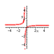
We can type in the expression that defines the slope of the tangent or derivative of G at a=-1/4.

> Limit((G(-1/4+h)-G(-1/4))/h,h=0);

>

> value(%);

At the point (-1/4,-1/2) the equation of the tangent line is y=4x+1/2. We can plot G together with its tangent line to see if it looks correct:

> plot({G(x),4*x+1/2},x=-3..3,y=-5..5,color=black);

>

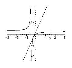
We could just use MAPLE's built in command "D" for calculating the derivative of a function at a point:

> D(G);

> D(G)(-1/4);

If we use the expression form of G, namely G(x), then the syntax is "diff" not "D" and to evaluate one needs to use the subs command:

> diff(G(x),x);

> subs(x=-1/4,diff(G(x),x));