Pattern Formation and Partial Differential Equations
Abstract: In this course, I will discuss three partial differential equations (PDE) that model pattern formation. Numerical simulations reveal that solutions of these deterministic equations have indeed stationary or self-similar statistics, which are independent of the system size and of the details of the initial data. We show how PDE methods can be used to understand some aspects of this universal behavior.
The first PDE has the structure of a gradient flow (a feature on which the analysis relies), the second PDE has the structure of a driven gradient flow, whereas the third PDE is half-way between a conservative and a dissipative system.
1. Bounds on the coarsening rate in spinodal decomposition
The PDE -- the Cahn-Hilliard equation -- is given by
Numerical simulations reveal that for generic initial
data (e. g. small amplitude white noise) after an initial layer, ![]() divides into
a convoluted domain where
divides into
a convoluted domain where ![]() and its complement where
and its complement where ![]() ,
separated by a characteristic interfacial layer of width
,
separated by a characteristic interfacial layer of width ![]() . This
domain configuration coarsens over time. More precisely, the average
length scale of the domains behaves as
. This
domain configuration coarsens over time. More precisely, the average
length scale of the domains behaves as ![]() .
This is reflected by the fact that the average energy per volume, i. e.
.
This is reflected by the fact that the average energy per volume, i. e.
![]() ,
behaves as
,
behaves as ![]() .
.
We shall prove that, in a time-averaged sense,
![]() .
This is joint work with R. V. Kohn.
.
This is joint work with R. V. Kohn.
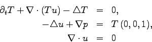
2. Bounds on the Nusselt number in Rayleigh-Bénard convection
The system of PDEs is given by an advection-diffusion equation for the
temperature ![]() ,
and the Stokes equations with buoyancy for the fluid velocity
,
and the Stokes equations with buoyancy for the fluid velocity ![]() , i. e.
, i. e.
Experiments and numerical simulations for ![]() show a
chaotic velocity field
show a
chaotic velocity field ![]() , with regions of high temperature
, with regions of high temperature ![]() in
form of mushrooms (plumes). This leads to a high upwards
heat transport -- much higher than the one mediated by diffusion allone.
This upwards heat flux is given by the Nusselt number
in
form of mushrooms (plumes). This leads to a high upwards
heat transport -- much higher than the one mediated by diffusion allone.
This upwards heat flux is given by the Nusselt number
![]() .
Experiments and asymptotic analysis suggest that
.
Experiments and asymptotic analysis suggest that ![]() .
.
With the help of the background field method, we will prove
that indeed ![]() in
in ![]() (up to a logarithm).
This is joint work with C. Doering and M. Reznikoff-Westdickenberg.
(up to a logarithm).
This is joint work with C. Doering and M. Reznikoff-Westdickenberg.
3. Bounds on the average dissipation in the Kuramoto-Sivashinsky equation
The PDE -- the Kuramoto-Sivashinsky equation -- is given by
For ![]() ,
numerical simulations reveal that the solutions have
an average length scale of
,
numerical simulations reveal that the solutions have
an average length scale of ![]() , and an average
amplitude of
, and an average
amplitude of ![]() and display spatio-temporal chaos.
and display spatio-temporal chaos.
We will argue that the average dissipation rate,
i. e.
![]() ,
is
,
is ![]() in
in ![]() (up to a logarithm). The argument relies on a new
observation
on the inhomogeneous inviscid Burger's equation
(up to a logarithm). The argument relies on a new
observation
on the inhomogeneous inviscid Burger's equation