Next: Applications to Fluid Dynamics
Up: Introduction to Shape Design
Previous: Control Problems Governed by
We consider next problems in which the design variable is the shape of the
domain in which a PDE is given. We need to derive formulas for the changes
of different cost functionals which depend on the shape.
Let us take some examples of practical importance.
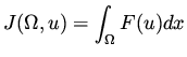
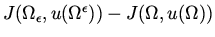
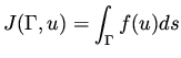
Example I: The functional depends on the whole domain.
Consider the functional
 |
|
|
(47) |
which depends on the domain as well as on a function
 , which
depends on that domain too. For the moment we do not specify exactly
the dependence of this function on the domain. Later on this function will
be a solution of a PDE defined in
, which
depends on that domain too. For the moment we do not specify exactly
the dependence of this function on the domain. Later on this function will
be a solution of a PDE defined in  , and will change as
we change the domain .
, and will change as
we change the domain .
We need to calculate the variation of this functional with respect to .
To do this we assume that the function  is defined in a
slightly larger domain that includes .
We examine
is defined in a
slightly larger domain that includes .
We examine
 where
where
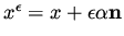
 is a small perturbation of ,
parameterized by a small number
is a small perturbation of ,
parameterized by a small number  .
The perturbation of the shape is done following Pironneau [13].
The boundary of is perturbed
in the direction of the outward normal to by
.
The perturbation of the shape is done following Pironneau [13].
The boundary of is perturbed
in the direction of the outward normal to by
 , where
  is a parameterization of the
boundary,
is a parameterization of the
boundary,  is the outward normal and
  is an arbitrary
function defined on the boundary. We use the short notation,
is an arbitrary
function defined on the boundary. We use the short notation,
 and
.
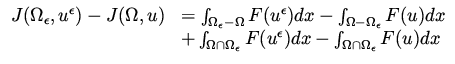
We have
and
.
We have
 |
|
|
(48) |
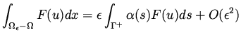
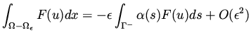
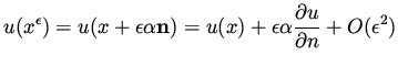
For small these integrals can be approximated
as follows
where
![$\displaystyle \tilde u = \lim _{\epsilon \rightarrow 0} \frac{1}{\epsilon}[u^\epsilon - u]$](img123.png) |
|
|
(52) |
and
 and
and
 .
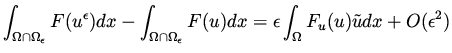
We conclude that,
.
We conclude that,
![$\displaystyle \frac{1}{\epsilon} [ J( \Omega _\epsilon ) - J( \Omega) ] = \int _{\Gamma } \alpha (s) F(u) ds + \int _\Omega F_u(u)\tilde u ds + O ( \epsilon).$](img126.png) |
|
|
(53) |
This formula is useful when we have functionals defined on the interior of the
domain up to the boundary. Recall that in order to construct the necessary
conditions, or to calculate gradients, we need to consider this type of
expression.
Example II: Boundary Functionals.
Consider next the functional
 |
|
|
(54) |
where
 ,
,  is an area element, and
  is part of
the boundary of a domain . The function
is part of
the boundary of a domain . The function  depends on the domain in a way which we do not
prescribe at the moment.
Again we are interested in perturbations of the domain, and as a result of
it perturbations of . It is convenient to use the same type of
perturbation as before.
The new boundary will be denoted by
depends on the domain in a way which we do not
prescribe at the moment.
Again we are interested in perturbations of the domain, and as a result of
it perturbations of . It is convenient to use the same type of
perturbation as before.
The new boundary will be denoted by
 and we want to calculate
![$\displaystyle \frac{1}{\epsilon} [J( \Gamma _\epsilon , u^\epsilon ) - J( \Gamma ,u) ]$](img132.png) |
|
|
(55) |
for small . This case is slightly more complicated since
we have to consider the change of the area element as well.
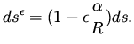
Consider a line element ,
where the radius of curvature is given by  .
Note that this line element can be
written as
.
Note that this line element can be
written as  where is the radius
of curvature and
where is the radius
of curvature and  represent an infinitesimal angle. A change in the
boundary by
represent an infinitesimal angle. A change in the
boundary by
 changes the line element
to
changes the line element
to
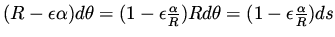 .
Thus, we obtain a formula, for the two dimensional case, for the new line
element
.
Thus, we obtain a formula, for the two dimensional case, for the new line
element
 |
|
|
(56) |
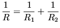
For problem in three dimension we consider two orthogonal
tangential coordinates and in
each direction a similar result hold for the line element. The area
element being the product of the two line elements has the formula (56) but
now with
 |
|
|
(57) |
where  and
and  are the radiuses of curvature
in two orthogonal directions on the
surface. Note that the quantity
are the radiuses of curvature
in two orthogonal directions on the
surface. Note that the quantity  does not depends on the choice
of coordinate system since it is the trace of the matrix of second derivatives of the surface describing the boundary.
does not depends on the choice
of coordinate system since it is the trace of the matrix of second derivatives of the surface describing the boundary.
In order to obtain a simple expression for the variation of the functional
as a function of the boundary we have to express
 in terms of an integral and quantities on .
Consider a point  and the corresponding shift of it to
 given by
 .
The integral depends on which is a function of
.
The integral depends on which is a function of  , and
, and
 |
|
|
(58) |
 |
|
|
(59) |
For simplicity, we assume that  does not depends explicitly on , although this can
be handled as well. Using the last two formulas we have
does not depends explicitly on , although this can
be handled as well. Using the last two formulas we have
 |
|
|
(60) |
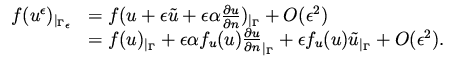
Using this together with the formula for the line (area) element (56) we get
![$\displaystyle \begin{array}{ll}
f(u^\epsilon ) ds ^\epsilon & = (f(u) + \epsilo...
...alpha }{R} f(u) ] ds + \epsilon f_u(u) \tilde u ds + O(\epsilon ^2)
\end{array}$](img152.png) |
|
|
(61) |
Substituting (61) into (55) we have
 |
|
|
(62) |
Next: Applications to Fluid Dynamics
Up: Introduction to Shape Design
Previous: Control Problems Governed by
Shlomo Ta'asan
2001-08-22