


Next: Bibliography
Up: Applications to Fluid Dynamics
Previous: Shape Design Using The
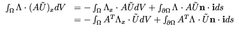
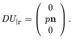
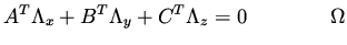
Our next example is a similar minimization problem but this time subject to the
Euler equation. Namely,
 |
|
|
(82) |
where  , and
, and  is the solution of the Euler equation.
Here stands for the variables
is the solution of the Euler equation.
Here stands for the variables
 and
and
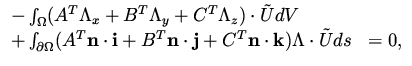
 . The Euler equations in conservation form are written as
 |
|
|
(83) |
where
 |
|
|
(84) |
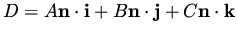
and
where the matrices  can be found, for example, in Hirsch [12].
An important property of the equation that we use here is
can be found, for example, in Hirsch [12].
An important property of the equation that we use here is
 |
|
|
(85) |
The change  in the flux vector
  satisfies,
 |
|
|
(86) |
and similar expressions for
 .
The equation for the perturbation quantities reads
.
The equation for the perturbation quantities reads
 |
|
|
(87) |
or equivalently,
 |
|
|
(88) |
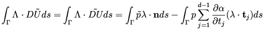
Now consider the following identity which follows from integration by parts,
 |
|
|
(89) |
and similar integrals for the  and
and  terms.
Combining these identities we arrive at
terms.
Combining these identities we arrive at
 |
|
|
(90) |
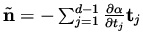
for an arbitrary  .
We will use the notation
.
We will use the notation
 |
|
|
(91) |
and note that  is the normal flux at the boundary
which has the form, see Hirsch [12],
is the normal flux at the boundary
which has the form, see Hirsch [12],
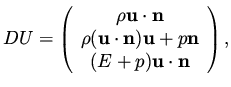 |
|
|
(92) |
and at a wall where
 , it reduces to
 |
|
|
(93) |
We have
 following (84),(86) and its analog for the
terms, and
following (84),(86) and its analog for the
terms, and
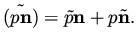 |
|
|
(94) |
Combining the last equalities and
 from (75),
we get
from (75),
we get
 |
|
|
(95) |
where we used the notation
 , and
, and
 .
The wall boundary condition
.
The wall boundary condition
 |
|
|
(96) |
becomes upon perturbation
 |
|
|
(97) |
and as before we transfer this boundary condition to the original boundary
 ,
,
 |
|
|
(98) |
Collecting only the  terms we get
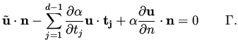 |
|
|
(99) |
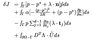
The variation of the functional
![$\displaystyle \delta J = \int _{\Gamma} [ (p - p^*) \tilde p + \alpha (p - p^*) \frac{\partial p}{\partial n}- \alpha \frac{(p-p^*)^2}{2R} ] ds$](img223.png) |
|
|
(100) |
will be simplified by adding (90) to it,
but with a choice of which makes the volume integral vanish.
Thus, we assume that
 |
|
|
(101) |
Using (90),(95) it leads to
 |
|
|
(102) |
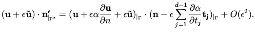
Now we come to use the boundary conditions for  .
We begin with the far field
.
We begin with the far field
 . We assume that the
boundary conditions there are given in terms of characteristic variables and assume
that
. We assume that the
boundary conditions there are given in terms of characteristic variables and assume
that
 is the matrix such that
  are the characteristic
variables.
We write the far field term as
are the characteristic
variables.
We write the far field term as
 |
|
|
(103) |
We distinguish the following cases.
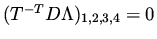
Supersonic inflow: all variables are specified at inflow, and thus  .
Thus, no boundary conditions are imposed on .
Supersonic outflow: No boundary conditions are specified for , hence
is arbitrary there and therefore we are led to the choice
.
Thus, no boundary conditions are imposed on .
Supersonic outflow: No boundary conditions are specified for , hence
is arbitrary there and therefore we are led to the choice
 at supersonic outflow.
Subsonic inflow: 4 conditions are specified (3 in 2D), and those are
at supersonic outflow.
Subsonic inflow: 4 conditions are specified (3 in 2D), and those are
 ,
thus
,
thus
 is arbitrary, leading to
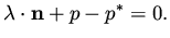
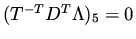 . Subsonic outflow: one condition is given
for
which implies
. Subsonic outflow: one condition is given
for
which implies
 and therefore
 .
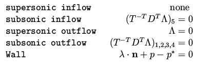
On the wall we choose
.
On the wall we choose
 |
|
|
(104) |
In summary, the boundary conditions for are
 |
|
|
(105) |
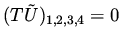
With this choice for together with the interior equation (101) we
get that  involves integrals depending on
  and
and not on terms.
Rearrangement by using integration by parts gives,
and
and not on terms.
Rearrangement by using integration by parts gives,
![$\displaystyle \delta J =
\int _\Gamma \alpha [- \frac{(p-p^*)^2}{2R} + (p-p^*) \frac{\partial p}{\partial n}-div (p \lambda )]ds.$](img238.png) |
|
|
(106) |
The gradient of the functional in this case is therefore given by
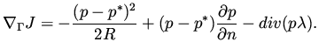 |
|
|
(107) |
Next: Bibliography
Up: Applications to Fluid Dynamics
Previous: Shape Design Using The
Shlomo Ta'asan
2001-08-22