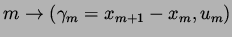
Congestion on Multilane Highways
Introduction
All computations in this section were run with the following equilibrium relations:
 |
(1) |
These transform to
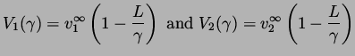 |
(2) |
where
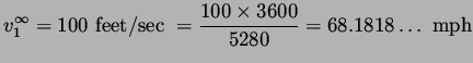
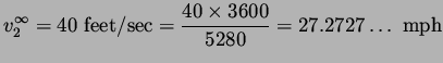
 . The specific parameter used were
 |
(3) |
 |
(4) |
and
 |
(5) |
The latter number corresponds to a maximum car density of
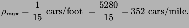 |
(6) |
We used the constant switch curve introduced by Sopasakis [1]:
 |
(7) |
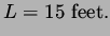
with
 feet. For initial data we chose 3 sets
of data:
feet. For initial data we chose 3 sets
of data:
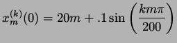 |
(8) |
for
 and
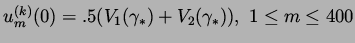
and  , and 3. The observation that
 |
(9) |
and
 |
(10) |
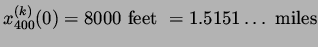
implies we may interpret the data as initial data for a ring-road with 400 cars which is of length 1.5151... miles. We chose constant initial velocities
 |
(11) |
or
 |
(12) |
These data guarantee points on both sides of the switch curve. Simulations were run with relaxation times
 |
(13) |
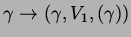
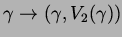
A word is inorder about the simulations which follow. The first two frames in each figure are self-explanatory. In the third frame of each figure we plot the curve
 . This curve is shown in black. The blue curves are the equilibrium curves
 and
and
 and the red curve is the image of
 . The red dot - o - is the image of
 . The discontinuities in the profiles propagate at the speed
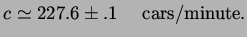 |
(3.14) |
Simulation
Downloads
Lagrangian Representation source code
Eulerian Representation source code
Paper (ps)
Paper (pdf)
Pei-Jen Lin
2001-08-22